Properties of physical bodies and objects opi physical quantities . One of these quantities for electric field is an tension. In accordance with the previously defined definition, it describes the power action of the field at the dawn-feminine bodies at a specific point of the electric field. If the field is inhomogeneous, then the tension at different points of the field is different. And in order to describe the properties of the field in many points, it is necessary to submit a large number of tension values. This must-fighters the study of the field and prevents the creation of a presentation of a person in each particular case in the imagination.
The electric field strength is its power characteristics.
It is better to represent the structure of the electric field helps graphic method. At the basis of the graphical representation method electric field structures There are re-alleged phenomena that can be observed in experiments.
Let B electric field A positive-charged ball has a small particle of a substance, also having a polo charge. If this partial is free and the action of the gravitational field is not significant, then under the influence of electricity, it will move from the ball. This will be observed anywhere in the field of the charged ball (Fig. 4.20).
Posing the trajectory of the movement of many positively charged particles, which is in the electric field, and pointing on them the direction of the current force, a semi-chim picture called spectrum This field.
The lines forming the spectrum of the electric field are called lines of tensionelectric field, or silent lines.
Concept force line For the first time introduced into science M. Faraday based on the knowledge obtained during the experimental examinations.
Experiments, famous M. Faraday, can be implemented in modern conditions.
Take a metal conductor with a paper strip-fastened to it and connect it with a conductor of an electrophore machine. If we give it into action, then all the strips of paper will differ in different directions as a result of mutual from-pin (Fig. 4.21). The results of this experience (and similar to it) allow the post-digit of the electrical field of a separate charged body. It is shown in Fig. 4.22. The arrows on the power lines are shown the direction of force that will act on a positively charged body located at this point point.
Therefore, the power lines "exit" from a positively charged body and "enter" into a negatively charged body (Fig. 4.22). At the same time, it should be remembered that they "exhausted" and "enter" perpendicular to the surface of the body.
The lines of electrical intensity are perpendicular to the surface of the charged body at those points where they start. Material from site.
Take two metal conductor with paper stripes and connect them with the conductor of the electrophore machine. At the time, the electrolyte machine and we will see that the paper strips will start at one to each other (Fig. 4.23). According to the two variemlessly charged bodies, the field of two different charged bodies will have a spectrum shown in Fig. 4.24.
The curvilinear form of lines of tension is due to the fact that there are two forces from each body on the side of each body. The equilment of these forces at each point of the field is tangent to the lines of tension.
Lines tangents to which at any point show the direction of force acting on a positively charged point body called lifesty.
The directions of forces that will be valid at different points of the field of two dust-feminine bodies are shown in Fig. 4.25.
Since tension lines are always perpendicular to the surface, the spectra of body fields of various forms will be different (Fig. 4.26).
On this page, material on the themes:
Email spectra. fields of various charged bodies
Graphic image of the electrical field Abstract
Images of lines of electric fields on experiments
-
For greater clarity, the electric field is often depicted using power lines and equipotential surfaces.
Power lines – these are continuous lines tangents to which at each point through which they pass, coincide with the vector of electric field strength (Fig. 1.5). The thickness of the power lines (the number of power lines passing through the unit area) is proportional to the electric field strength.
Equipotential surfaces (equipotential) – surfaces of equal potential. These are surfaces (lines), when driving on which the potential does not change. Otherwise, the potential difference between two any points of the equipotential surface is zero. Power lines Perpendicular to the equipotential surfaces and are directed towards the most sharp decrease of potential. This fact follows from equation (1.10) and proves in the course of mathematical analysis by the section "Scalar and Vector Fields".
Consider the electrical field created at a distance
 from point charge. According to (1.11, b) tension vector coincides with the direction of the vector
  If the charge is positive, and is opposite to him if the charge is negative. Consequently, the power lines are diverted radially from charge (Fig. 1.6, a, b). Thickness of power lines, as well as tensions, inversely proportional to the square of the distance (
  ) Before charge. The equipotential surfaces of the electric field of a point charge are spheres with a center at the location of the charge.
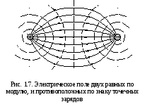
In fig. 1.7 shows the electrical field of the system of two equal in the module, but opposed to the sign of point charges. We provide to make out this example readers on their own. We only note that the power lines always begin on positive charges and ends on negative. In the case of an electrical field of one point charge (Fig. 1.6, a, b) it is assumed that the power lines are broken on very remote charges of the opposite sign. It is believed that the universe is generally neutral. Therefore, if there is a charge of one sign, then somewhere I will definitely have an equal one in the module of the charge of another sign.
1.6. Gaussian Theorem for Electric Field in Vacuum
The main task of electrostatics is the task of finding the tension and the potential of the electric field at each point of space. In paragraph 1.4, we decided the task of the field of a point charge, and also considered the field of a system of point charges. In this paragraph, it will be about the theorem that allows you to calculate the electrical field of more complex charged objects. For example, a charged long thread (straight), charged plane, charged sphere and others. Calculating the electric field strength at each point of space using equations (1.12) and (1.13), it is possible to calculate the potential at each point or the potential difference between the two any points, i.e. Solve the main task of electrostatics.
For a mathematical description, we introduce the concept of stream of tension or electric field stream. Stream (f) vector
 electric field through a flat surface area
  called the value:
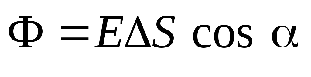 ,
(1.16)
,
(1.16)
where
 - electric field strength, which is expected to constant within the site ;
 - angle between the direction of the vector and single vector normal
  to the site (Fig. 1.8). Formula (1.16) can be recorded using the concept of a scalar product of vectors:
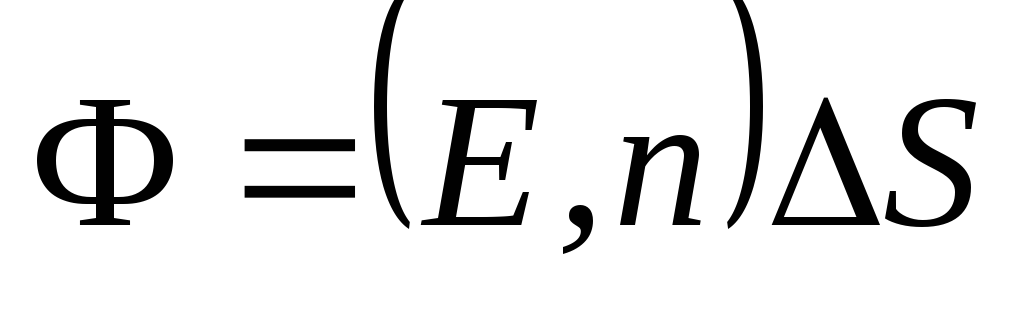 . (1.15, a)
In the case when the surface
 not flat, it must be divided into small parts to calculate the stream
  which can be approximately considered flat, and then record expression (1.16) or (1.16, a) for each piece of surface and fold them. In the limit when the surface S. i. very small
  ), such an amount is called superficial integral and denote
 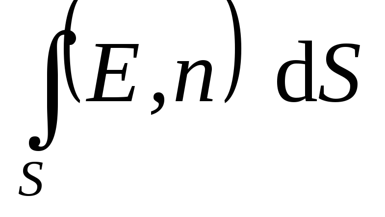 . Thus, the flow of the electric field strength vector through an arbitrary surface determined by the expression:
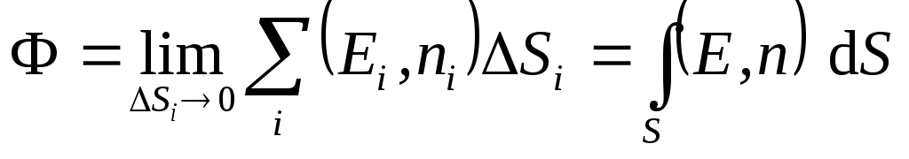 .
(1.17)
.
(1.17)As an example, consider the sphere of radius
, which is the center of which is a positive point charge  and we define the flow of the electric field through the surface of this sphere. Power lines (see, for example, Fig.1.6, a) emerging from charge, perpendicular to the surface of the sphere, and at each point of the sphere the field strength module is the same
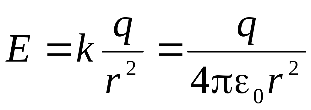 .
.Square sphere
 ,
,then

 .
.Value
 and is a flow of an electric field through the surface of the sphere. Thus, we get
  . It can be seen that the flow through the surface of the sphere of the electric field does not depend on the radius of the sphere, and it depends only on the charge itself . Therefore, if you hold a number of concentric spheres, the flow of the electric field through all these areas will be the same. It is obvious that the number of power lines crossing these spheres will also be the same. The number of power lines coming out of charge, taking an equal stream of the electric field:
  .
.If the sphere is replaced by any other closed surface, then the flow of the electric field and the number of power lines crossing it will not change. In addition, the flow of the electric field through a closed surface, and therefore the number of power lines penetrating this surface is equal to
 not only for a point of point charge, but also for a field created by any combination of point charges, in particular, a charged body. Then magnitude it should be considered as an algebraic amount of the entire totality of charges inside a closed surface. This is the essence of the Gauss Theorem, which is formulated as follows:
Electric field strength vector stream through arbitraryclosed the surface is equal
where
algebraic
The amount of charges concludedinside
this surface.
algebraic
The amount of charges concludedinside
this surface.Mathematically theorem can be written as
 .
(1.18)
.
(1.18)Note that if on some surface S. vector
 permanent and parallel vector
  , then flow through such a surface. Converting the first integral, we first used the fact that the vectors and parallel, which means
  . Then they delivered the amount for the sign of the integral due to the fact that it is constant anywhere in the sphere . Using the Gaussory Theorem to solve specific tasks, it is trying to select the surface for which the conditions described above is trying specifically as an arbitrary closed surface.
We give several examples to apply Gauss theorem.
Example 1.2.Calculate the electric field strength of a uniformly charged endless thread. Determine the potential difference between two points in such a field.Decision. Suppose to certainty that the thread is charged positive. By the symmetry of the task, it can be argued that the power lines will be radially divergen from the axis of the thread straight (Fig.1.9), the density of which is reduced from the thread to some law. The magnitude of the electric field will decrease on the same law.
 . Equipotential surfaces will be cylindrical surfaces with the axis that coincides with the thread.
Let the charge unit of the length of the thread equal
 . This value is called a linear charge density and is measured in SI in units [CL / M]. To calculate the field strength, apply Gauss theorem. To do this, as an arbitrary closed surface choose a radius cylinder and length
  whose axis coincides with the thread (Fig.1.9). Calculate the flow of the electric field through the surface area of \u200b\u200bthe cylinder. Full stream consists of a stream through the side surface of the cylinder and flow through the base
But,
 because at any point on the bases of the cylinder
  . It means that
  at these points. Stream through the side surface
  . According to the Gauss Theorem, this complete flow is equal
  . Thus, got
 .
.The amount of charges inside the cylinder, express through the linear density of the charge
: . Considering that
  , get
, get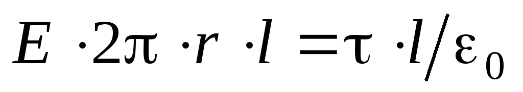 ,
,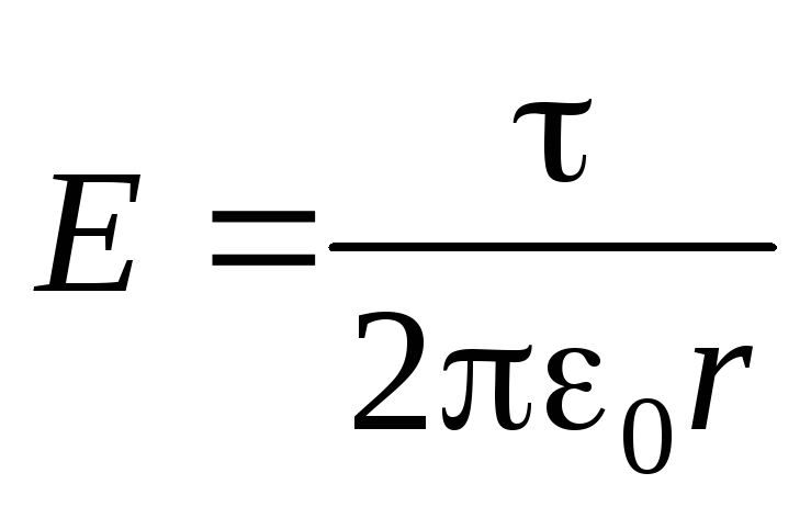 ,
(1.19)
,
(1.19)those. The tension and density of the power lines of the electric field of a uniformly charged endless thread decreases inversely proportional to the distance (
 ).
).Find the potential difference between points located at distances
 and
and  from thread (owned by equipotential cylindrical surfaces with radii and ). To do this, we use the tension of the electric field with the potential in the form (1.9, B):
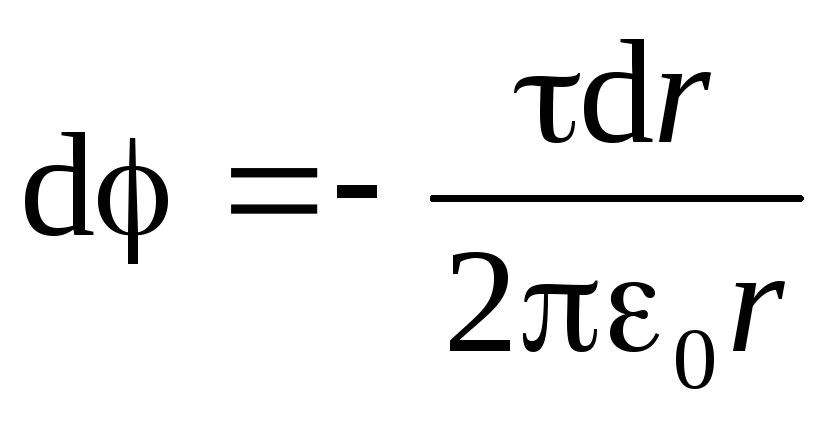
  . Given the expression (1.19), we obtain a differential equation with separating variables:
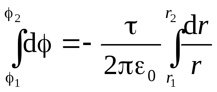
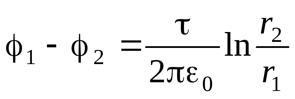 .
.
Example 1.3.Calculate the electric field strength of a uniformly charged plane. Determine the potential difference between two points in such a field.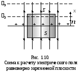
Decision. The electrical field of a uniformly charged plane is shown in Fig. 1.10. By virtue of symmetry, the power lines must be perpendicular to the plane. Therefore, it can immediately conclude that the thickness of the lines, and, consequently, the tension of the electric field when removing the plane will not change. Equipotential surfaces are planes parallel to this charged plane. Suppose the charge unit of the plane area is equal
 . This value is called the superficial charge density and is measured in C in units [CL / m 2].
Apply Gauss theorem. To do this, as an arbitrary closed surface
choose a cylinder length  , whose axis is perpendicular to the plane, and the bases are equidistant from it (Fig.1.10). Total electric field stream
  . The flow through the side surface is zero. Flow through each of the base is equal
  , so
, so  . According to the Gauss theorem, we get:
 .
.The sum of charges inside the cylinder
we will find through the superficial density of the charge : . Then, Location:
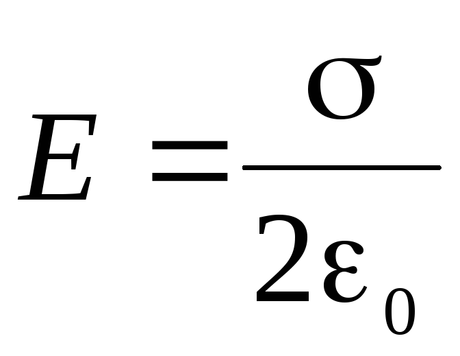 .
(1.20)
.
(1.20)From the resulting formula, it can be seen that the intensity of the field of a uniformly charged plane does not depend on the distance to the charged plane, i.e. At any point of space (in one half-plane) is the same and module, and in the direction. This field is called uniform. Power lines uniform field Parallel, their density does not change.
Find the potential difference between two points of a homogeneous field (owned by equipotential planes
 and
and  lying in one half-plane relative to the charged plane (Fig.1.10)). We direct the axis
  vertically upwards, then the projection of the tension vector on this axis is equal to the modulus of the tension vector
  . We use equation (1.9):


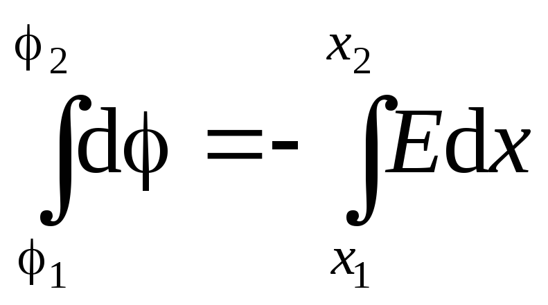 .
.Permanent quantity
(Uniformly) can be taken out of the integral sign: 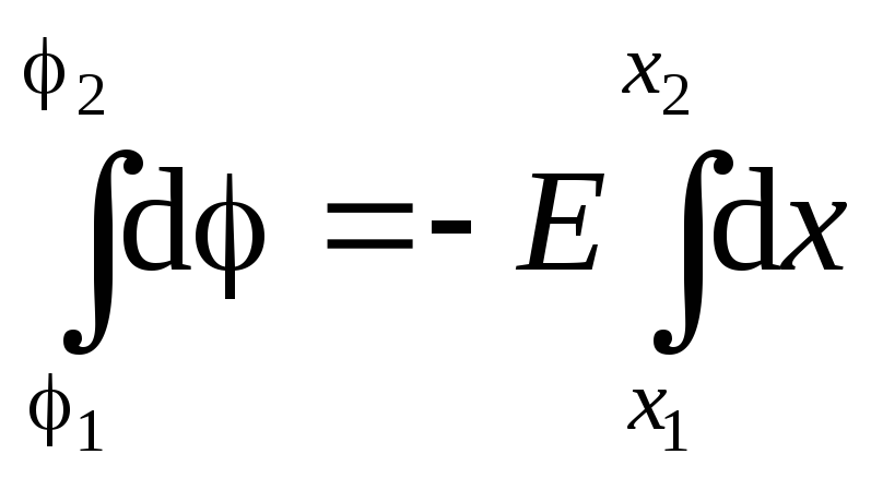 . Integrating, we get :. So, the potential of a homogeneous field linearly depends on the coordinate.
The difference of potentials between the two points of the electric field - there is a voltage between these points (
 ). Denote the distance between the equipotential planes
  . Then it can be written that in a uniform electric field:
 .
(1.21)
.
(1.21)We emphasize once again that when using formula (1.21) you need to remember that the value
Example 1.4.Calculate the electric field strength of two parallel planes, uniformly charged with surface densities of charges Not the distance between points 1 and 2, and the distance between the equipotential planes, which these points belong.
 and
and  .
.Decision. We use the result of Example 1.3 and the principle of superposition. According to this principle, the resulting electric field at any point of space
 where
where  and
and  - Electric fields of the first and second plane. In space between the planes of the vector and directed in one direction, so the reference field strength module. In the external space vector and directed in different directions, therefore (Fig. 1.11). Thus, the electric field is only in space between the planes. It is homogeneously, since it is the sum of two homogeneous fields.
Example 1.5. Find the tension and potential of the electric field of a uniformly charged sphere. The total charge of spheres is equal
 , and the radius of the sphere -
  .
.Decision. Due to the symmetry of the charge distribution, power lines should be directed along the radii of the sphere.
Consider the area inside the sphere. As an arbitrary surface
choose the sphere of radius  , the center of which coincides with the center of the charged sphere. Then the flow of the electric field through the sphere S.:
 . The amount of charges within the sphere radius equal to zero, since all charges are located on the surface of the radius sphere
  . Then on the Gauss Theorem:
  . Insofar as
  T.
T.  . Thus, inside the uniformly charged field of the field.
Consider the area outside the sphere. As an arbitrary surface
choose the sphere of radius  , the center of which coincides with the center of the charged sphere. Stream of electric field through the sphere :. The amount of charges within the sphere is equal to the full charge charged Radius Sphere . Then on the Gauss Theorem:
 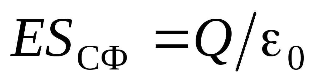 . Considering that
 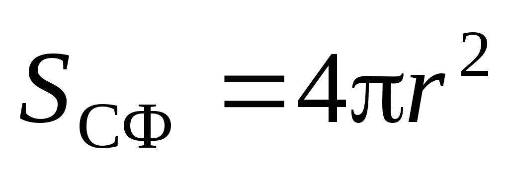 We will get:
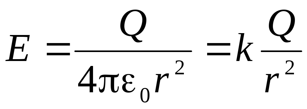 .
.Calculate the potential of the electric field. It is more convenient to start with the outside
As we know that at an endless distance from the center of the sphere, the potential is taken equal to zero. Using equation (1.11, a) we obtain a differential equation with separating variables: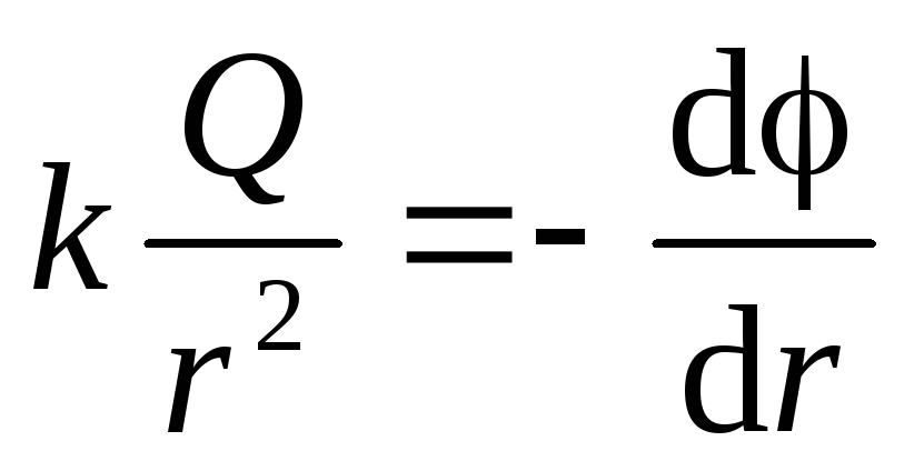


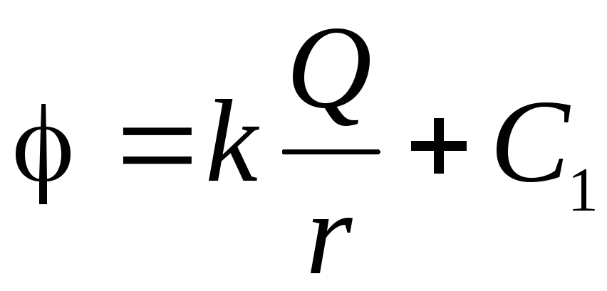 .
.Constant
 , insofar as
  for
for  . Thus, in the external space ( ):
 .
.Points on the surface of the charged sphere (
 ) will have the potential
  .
.Consider the area
. In this region , therefore, from the equation (1.11, a) we get: 

 . Due to the continuity of the function
  constant
  must be equal to the value of the potential on the surface of the charged sphere:
  . Thus, the potential at all points within the sphere:
  .
.
So, we obtained that the tensions and potential of the electric field created by a uniformly charged sphere, outside the sphere are equal to the tension and the potential of the field created point charge of the same magnitude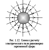 As the charge of spheres placed in the center of the sphere. In inner space The field is absent, and the potential at all points is the same. The electric field (power lines and the equipotential surfaces) of the charged sphere are shown in Fig. 1.12. It is assumed that the sphere is charged positively. Outside the sphere of power lines and distributed in space in the same way as the power lines of the point charge.
In fig. 1.13 depicts dependency graphics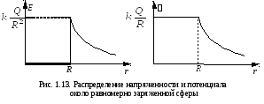
 and . Function continuous and function jumpingly changes when moving across the border of the charged sphere. The magnitude of the jump is equal
  . Indeed, near the charged sphere (
  ) field strength in external space
  , and inside is zero.
The magnitude of the jump can be expressed through the surface density of the charge on the sphere:
 .
.Note that this is the overall property of the electrostatic field: on the charged surface, the projection of tension on the direction of normal is always leaving the jump
 regardless of the surface shape. We recommend checking this principle for the field of a uniformly charged plane and the fields of two parallel charged planes (examples 1.3, 1.4).
From the point of view of mathematics, the continuity of the potential at the points of the charged surface means that
 . From the point of view of physics, the continuity of the function
  can be explained as follows. If the potential on the border of some region would have a jump (break), then with an infinitely small movement of some charge from point 1 lying on one side of the border, to point 2, lying on another side, the final work would be performed
  where and Potentials of points 1 and 2, respectively, and the value
  equal to the magnitude of the rapid potential at the boundary of the region. The ultimate work, perfect on an infinitely small move, means that on the border of the partition would be infinitely large forces, which is impossible.
The electric field strength, in contrast to the potential, on the boundary of the region may vary very sharply (jumping).
Example 1.6.Two concentric spheres of radii
 and
and  (
( ) Equally charged with equal in the module, but opposite by the sign of charges
  and
and  (spherical condenser). Determine the tension and potential of the electric field in the entire space.
Decision. The solution to this problem could also begin with the use of the Gauss Theorem. However, using the results of the previous example and the principle of superposition (1.13, 1.14), the answer can be obtained faster.
At external points of space (
 ) The electric field is created by charges of both spheres. The magnitude of the field intensity of the first sphere
  and directed from spheres along radii. The magnitude of the intensity of the second sphere field is the same
  But the opposite is directed. Consequently, according to the principle of superposition, in all external points of space, the electric field will be absent
  .
.Consider the points of space between the spheres (
 ). These points are internal for a negatively charged sphere, so in this area
  (See Example 1.5). For a positively charged sphere, these points are external, so . Thus, the magnitude of the field strength in this area
  . Here the field creates only smaller charges.
Finally, in the inner points of space (
 )
) and So there is no electric field at these points.
Similarly, you can apply the principle of superposition and potentials. The following results are obtained:
:
 ;:
;:
 ;:
;:
 .
.We recommend independently getting these results, as well as schematically depict the electrical field and build graphs
and  .
.but b.
Knowing the tension vector of the electrostatic field at each of its point, you can present this field clearly using power lines of tension (vector lines
 ). Power lines of tension are carried out so that the tangent to them at each point coincided with the direction of the tension vector (Fig. 1.4, but).
The number of lines perpetifying the unit DS platform perpendicular to them are proportional to the vector module
(Fig. 1.4, b.).Power lines are attributed to the direction coinciding with the direction of the vector
. The resulting pattern of distribution of tension lines allows to judge the configuration of this electric field at different points. Power lines begin on positive charges And ends on negative charges.
In fig. 1.5 shows the line of strength of point charges (Fig. 1.5, but,
b.); systems of two variance charges (Fig. 1.5, in) An example of an inhomogeneous electrostatic field and two parallel variepelly charged planes (Fig. 1.5, g.) An example of a homogeneous electric field.1.5. Distribution of charges
In some cases, to simplify mathematical calculations, the true distribution of point discrete charges is conveniently replaced by a fictitious continuous distribution. During the transition to the continuous distribution of charges, the concept of charge density linear , surface and volumetric , i.e.
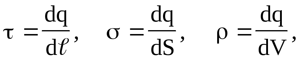 (1.12)
where DQ charge distributed according to the length element
 , Surface elementDs and DV volume element.
Taking into account these distributions of formula (1.11) can be recorded in another form. For example, if the charge is distributed in volume, then instead of q i need to use DQ \u003d DV, and the amount symbol is replaced by integral, then
 .
(1.13)
.
(1.13)1.6. Electric dipole.
To explain the phenomena associated with charges in physics, the concept is used Electric dipole.
The system of two equal in the magnitude of multi-dimensional point charges, the distance between which is much less than the distance to the studied points of space, is called an electric dipole. According to the definition of the dipole + q \u003d q \u003d q.
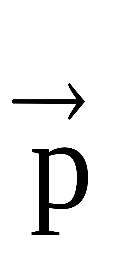
Direct connecting the variepete charges (poles) is called the dipole axis; Point 0 the center of the dipole (Fig. 1.6). Electric dipole is characterized shoulder dipole: Vector
 directed from the negative charge to the positive. The main characteristic of the dipole is electric dipole moment
 \u003d Q. .
(1.14)
\u003d Q. .
(1.14)In absolute value
p \u003d Q.
 .
(1.15)
.
(1.15)In X, the electric dipole moment is measured in the coulters multiplied by the meter (CL m).
Calculate the potential and tension of the electric field of the dipole, considering it point, if
r.The potential of the electric field created by the dot charge system in an arbitrary point characterized by the radius
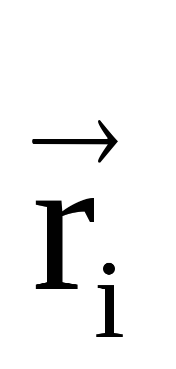 , Write in the form:
where R 1 R 2 R 2, R 1 R 2 r \u003d
 , as R; angle between radius-vectors
  and
and
 (Fig. 1.6) .
With this, we get
(Fig. 1.6) .
With this, we get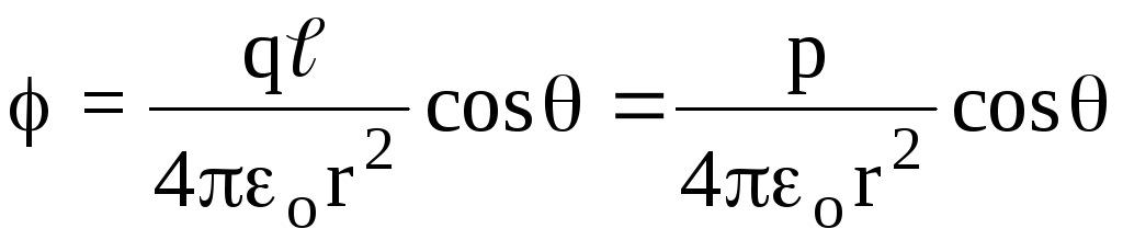 .
(1.16)
.
(1.16)Using a formula that connects the potential gradient with tension, we find the intensity created by the electric field of the dipole. Spider vector
 electric
dipole fields are two mutually perpendicular components, i.e.
electric
dipole fields are two mutually perpendicular components, i.e.  (Fig. 1. 6).
Their first of them is determined by the movement of the point characterized by the radius
(at a fixed value of the corner), i.e. the value of E Find differentiation (1.81) by R, i.e.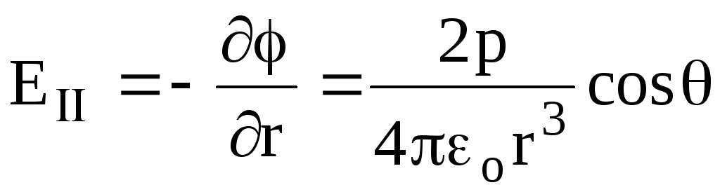 .
(1.17)
.
(1.17)The second component is determined by the movement of the point associated with the change in the angle (with a fixed R), i.e. E we find differentiation (1.16) by :
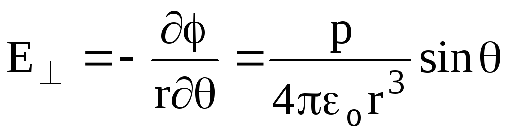 ,
(1.18)
,
(1.18)where
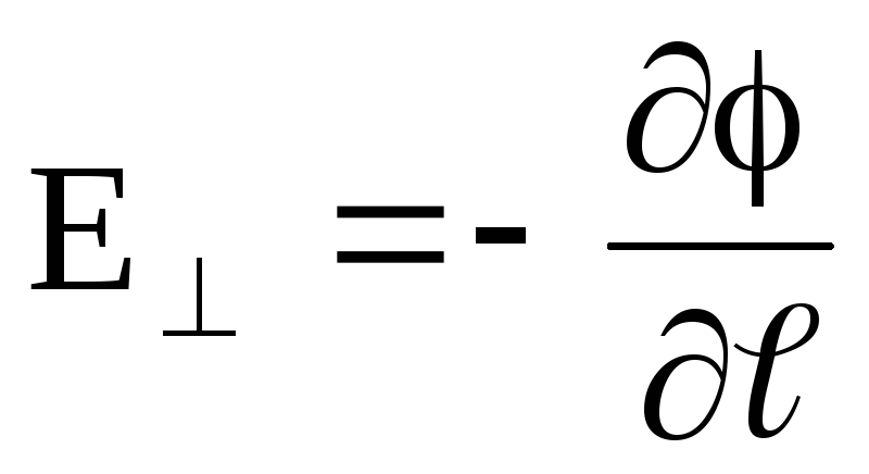 , D. \u003d RD.
Resulting tension E 2 \u003d E 2 + E 2 or after substitution
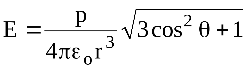 .
(1.19)
.
(1.19)Comment: At \u003d 90 o
 ,
(1.20)
,
(1.20)i.e. tension at the point on a straight line passing through the center of the dipole (T. O) and perpendicular to the axis of the dipole.
At \u003d 0
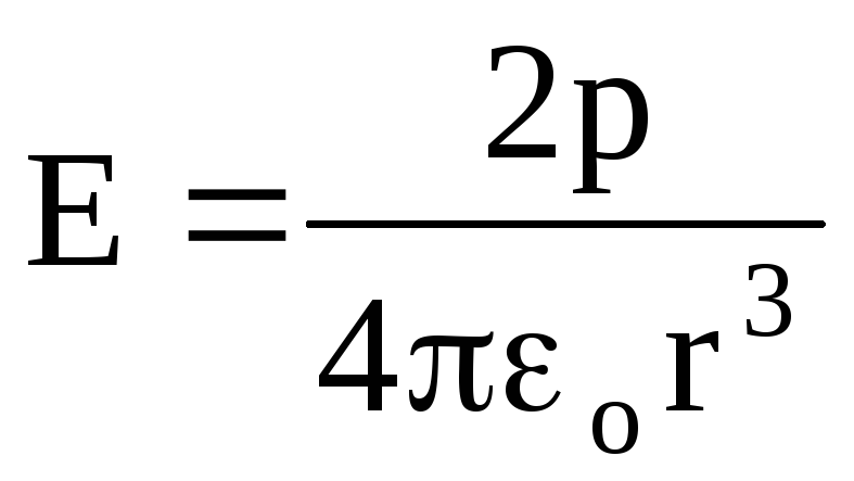 ,
(1.21)
,
(1.21)i.e. at the point on the continuation of the direct coinciding with the axis of the dipole.
Analysis of formulas (1.19), (1.20), (1.21) shows that the electric field strength of the dipole decreases with the distance inversely proportional to R 3, i.e. faster than for a point charge (inversely proportional to R 2).


