Consider the movement of the electron between the plane-parallel electrodes with distance D between them.
Laplace equation, having a view, after integration reduces to the equation
where u is the potential difference between the electrodes.
The electron motion equation in the rectangular coordinate system is divided into three equations:
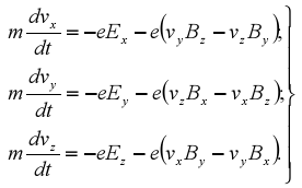
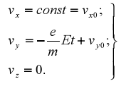
In the case under consideration, the magnetic field is absent, and the electrical has one component EY \u003d E. Then the system of equations will be recorded as
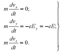
Suppose at the moment T \u003d 0, the electron is at the point of origin of the coordinates and moves with a velocity V0 having components along the x and y axes, and the speed component by z is zero. Then integration leads to equations:
After re-integrating the first two equations, we obtain;
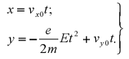
The integration constants in both cases are zero, since in the initial moment x \u003d y \u003d 0, the integration of the third equation gives z \u003d 0.
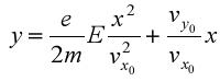
We obtain the equation of the electron trajectory, substituting:
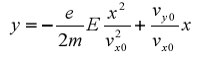
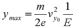
It can be seen that the movement occurs in parabole (curve 1 in Fig. 2.1) convexing upwards. Analysis shows that the peak of this parabola has coordinates
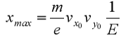
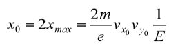
Making a move on this trajectory, the electron returns to the X axis at the point with the coordinate:
If the intensity vector is sent to the opposite direction (-U), the sign of the first member of the trajectory equation changes
those. In this case, the electron will move along the trajectory 2 (in Fig.2.1). This is a segment of parabola, symmetrical relative to the origin of Parabole coordinates 1.
\u003e Electron Movement in Accelerating Field
And and the image of the figure is depicted in the form silest lines (tension lines) a homogeneous electric field between two electrodes, such as a cathode and anode diode.
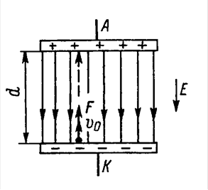
If the potential difference between the electrodes u , and the distance between them D , that field strength
For uniform field Value E.is constant.
Let from the electrode having a lower potential, for example, from the cathode TO,flies electron with kinetic energy W and initial speed V 0 , directed along the power lines of the field. The field accelerates the movement of the electron. In other words, the electron is attracted to the electrode with a higher potential. In this case, the field is called accelerating.
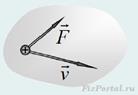
The field strength is numerically equal to force acting on a single positive charge. Therefore, the force acting on the electron
F. \u003d her.
The "minus" sign is supposed because the force F directed to the side opposite to the vector E.Sometimes this sign does not put.
Under the action of constant power f the electron is accelerated a \u003d f / t.Moving straight, electron acquires the greatest speed V and kinetic energy w at the end of its path, i.e. When hitting the electrode to which he flies. Thus, in the accelerating field, the kinetic electron energy increases due to the operation of the electron movement field. In accordance with the Law of Energy Conservation Increase kinetic energy electron W-W Equally, the work of the field, which is determined by the work of the charging charge e.on the potential difference passed by him:
W - W 0 \u003d mV 2 / 2 - MV 0 2 / 2 \u003d EU. (4)
If the initial electron speed is zero, then
W \u003d mV 2 / 2 \u003d EU. (5)
those. The kinetic electron energy is equal to the field of field.
Formula (5) with some approximation can be applied in the case when the initial speed v. 0 Many less ultimate speed v,as at the same time
mV 0 2 /2 " mV 2 /2
If it is conditionally adopted an electron charge per unit of amount of electricity, then at u \u003d 1 in electron energy is taken per unit of energy called electron-volt (eV). In most cases, it is convenient to express electron energy in electron-volt, and not in Joules.
Formula (5) determines the final electron rate
Substituting the meanings e and t,you can get a convenient expression for speed in meters or kilometers per second:
Thus, the electron speed in the accelerating field depends on the difference in potentials.
The initial energy of the electron is convenient to express in electron-volts, meaning equality
those. Considering that this energy is created by an accelerating field with the difference in potentials U 0.
Electron velocities Even with a small potential difference are significant. At u \u003d 1 in the speed is 600 km / s, and the app = 100 V - already 6000 km / s.
We will find T. T. electron span between electrodes, determining it with medium speed:
The average speed of the equilibrium movement is equal to the hemishemma of the initial and ultimate speeds:
If a , that
Substituting the value of the end speed, we get the time of the span in seconds:
here Distance D. expressed in meters, and if you express it in millimeters, then
For example, the time of the electron span at d \u003d3 mm and u = 100 B.
Due to the inhomogeneity of the field, the calculation of the time of the electron span in electronic devices is more complex. Almost this time is equal to. You can such a small time of flight in many cases not to take into account. But still, due to the fact that electrons have a mass, they cannot instantly change their speed and instantly flutter the distance between the electrodes. On ultra - and ultrahigh frequencies (hundreds and thousands of megahertz), the flight of an electron becomes commensurate with the period of oscillations. For example, at f \u003d 1000 MHz period T \u003d.from. The device ceases to be irregular or low-inertion. In other words, the inertia of electrons is manifested, which practically does not affect the work at low and high frequencies. At these frequencies, the oscillation period t a lot more of the flight of the electron and voltage variables on the electrodes during the flight do not have time to change significantly, i.e. It can be assumed that the electron span is performed at constant voltages of the electrodes.
Mode of operation for constant voltages of electrodes call static regime.When the voltage of at least one electrode changes so quickly that the laws of the static mode cannot be applied, the regime is called dynamic. If the voltages change with low frequency, so that the phenomena can be considered approximately with the help of the laws of the static regime, then the regime is called quasistatic.
Expressions for energy, speed and time span remain valid for any portion of the electron path. In this case, the magnitude W, V, T, D, Uapply only to this site.
If the field strength is different in different parts, the electron will fly with different acceleration in separate areas, and the final electron rate is determined only by the final potential difference and its initial speed. The law of conservation of energy implies that the final difference of potentials U.equal to the algebraic amount of the potential differences of individual sections. Therefore, the complete increment of kinetic energy is equal to the work eU.
In homogeneous electric field, The force acting on the charged particle is constant both in size and in the direction. Therefore, the movement of such a particle is completely similar to the body movement in the field of gravity of the Earth without taking into account air resistance. The trajectory of the particle in this case is flat, lies in the plane containing the veneer vectors of the particle and the electric field strength (Fig. 486).
fig. 486.
Therefore, to describe the position of the particle, two coordinates are sufficient. Conveniently one of the Cartesian axes of coordinates to send along the direction of the field strength vector (then the movement along this axis will be equal to the), and the second perpendicular to the intensity vector (movement along this axis is uniform). The beginning of the reference is conveniently combined with the initial position of the particle.
Simple example: mass particle m.bearing electric charge q. Moves in a homogeneous electric tension field E.at the initial moment its speed is equal v O.. Choose axis Oy. to the opposite vector direction E.The beginning of the reference is compatible with the initial position of the particle (Fig. 487). 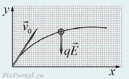
fig. 487.
Particle will move with constant acceleration
Directed "vertically down", so a further description of the movement, with all its features can be rewritten from solving the problem of body movement in the gravity field without taking into account air resistance.
Let's describe the principle of work electrostatic deflecting deviceused in a number of devices (for example, in some types of oscilloscopes) to change the direction of movement of the electron flow. Electron beam having speed v O., flies into the space between two parallel plates in length h.between which a constant electric field of tension has been created E.. On distance l. From the plates there is a screen to which this electron beam falls (Fig. 488). 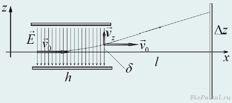
fig. 488.
Find the dependence of the beam deviation from the attached field strength.
We introduce the Cartesian coordinate system, as shown in Fig. 488. When the electrons moves between the plates on them there is a constant force F \u003d EE (e. - Electron charge, m. - His mass), which tells him acceleration a \u003d EE / MAxis Oz.. We will assume that the length of the plates is such that the electrons do not fall on it, moreover, we will neglect the edge effects, that is, we assume that the field between the plates is homogeneous, and there is no plates. Since the projection electric power on the axis is zero, then the projection of the speed on this axis does not change and remains equal v O.. During the span between the plates t 1 \u003d H / V O The electron will acquire an additional speed component directed along the axis Oy.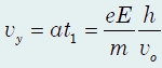
and shifts 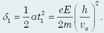
After departure from the field of the field, the electron will move evenly, so during the movement to the screen t 2 \u003d L / V O will additionally shift along the vertical axis to the distance 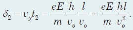
The total vertical offset of the stream will be equal to 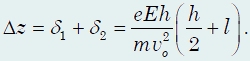
From this formula it follows that the displacement is proportional to the field strength, therefore, the difference in the potentials between deflecting plates. Thus, changing the voltage between the plates, you can change the position of the electron beam on the screen.
Chapter 29.
The movement of charges in electrical and magnetic fields
§ 1. Movement in homogeneous electric I magnetic fields
§ 2. Impulse analyzer
§ 3. Electrostatic lens
§ 4. Magnetic lens
§ 5. Electronic microscope
§ 6. Stabilizing accelerator fields
RepeatgL 30 (Vol. 3) "Diffraction".
§ 1. Movement in homogeneous electrical and magnetic fields
We now move on to the description in the general terms of the charges of charges in various conditions. The most interesting phenomena arise when charges move a lot and they all interact with each other. This is the case when electromagnetic waves pass through a piece of substance or plasma; Then the legions of charges interact with each other. But this is a very difficult picture. Later we will talk about such problems; In the meantime, we will discuss an incomparably simpler task about the movement of a separate charge in specifiedfield. At the same time, you can neglected by all other charges, except, of course, those charges and currents that create an estimated field.
It seems to begin, apparently, you need from the movement of the particle in a uniform electric field. Movement at low speeds does not represent much interest - it is simply evenly accelerated in the direction of the field. But when the particle, gaining enough energy, turns into relativistic, its movement becomes more complex. I leave you a solution for this incident to you - bother and find it yourself.
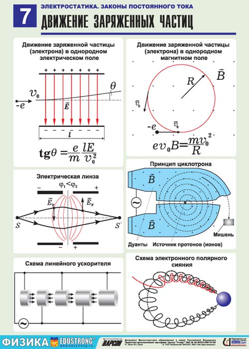
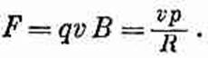
We will consider movement in a homogeneous magnetic field when there is no electric field. We have already solved this task. One of the solutions was the movement of particles around the circumference. Magnetic power
qV.X in always acts at right angles to the direction of movement, so the derivative dP / DT.perpendicular to p and equal in size vP / R,where R -radius of the circle, i.e.
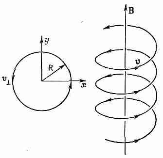
FIG. 29.1. Movement of particles in a homogeneous magnetic field.
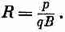
Thus, the radius of the circular orbit is equal
This is one of the possible movements. If the moving particle has only one component in the direction of the field, it does not change, because the magnetic force does not have a component in the field direction. The total movement of the particle in a homogeneous magnetic field is a movement with a constant speed in the direction of B and circular motion at a right angle to B, i.e., movement along the cylindrical helix (Fig. 29.1). The radius of the helix is \u200b\u200bdetermined by equality (29.1) with replacement ron the r + - pulse component perpendicular to field direction.
§ 2. Impulse analyzer
A homogeneous magnetic field is often used in the "analyzer", or the "pulse spectrometer" of high-energy particles. Suppose that at the point BUT(Fig. 29.2, but)in a homogeneous magnetic field, charged particles flies, and the magnetic field is perpendicular to the plane of the pattern. At the same time, each particle will fly along a circular orbit, the radius of which is proportional to its impulse. If all particles flies in the field perpendicular to its edge, then they leave it at a distance h.from the point BUT,proportional to their impulse r.Placed at some FROMthe counter will register only such particles whose impulse is somewhere in the range of DR values p \u003d QBX / 2.
FIG. 29.2. 180-degree spectrometer pulses with a homogeneous magnetic field.
a - particle trajectoriesfrom different impulses; 6.- the trajectories of particles flying at equal corners. The magnetic field is directed perpendicular to the plane of the pattern.
It is not necessary, of course, so that the particle is rotated 180 ° before registration, but such a "180-degree spectrometer" has a special property: it is very necessary for it that the particles come into at right angles to the edge of the field. FIG. 29.2, b.showing the trajectories of three particles with equestrianpulse, but included in the field at different angles. You see that they have different trajectories, but they all leave the field very close to the point FROM.In such cases, we are talking about "focusing". The advantage of this method of focusing is that it allows you to allow a point BUTalthough the particles flying at large angles, although usually, as seen from the drawing, these corners are to some extent limited. A large angular resolution usually means registration during this period of a larger number of particles and reduction, therefore, the measurement time.
Changing the magnetic field, moving the counter along the axis h.or covering with many meters a whole area along the axis x,you can measure the "spectrum" of the incident beam ["Spectrum" of pulses f (P)means that the number of particles with pulses in the interval between rand (P + DP)equal F (P) DP] . Such measurements are carried out, for example, when determining the distribution by energies in the B-decay of various cores.
There are still many other types of pulsed spectrometers, but I will tell you only about one of them, characterized by a particularly large resolution of spatialcorner. It is based on proper orbits in a uniform field, as shown in FIG. 29.1. Imagine a cylindrical coordinate system R, Q, Z, with the axis Z chosen in direction magnetic field. If the particle is emitted from the beginning of the coordinates at an angle
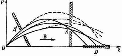
FIG. 29.3. Spectrometer with axial field.
and to the direction of the z axis, it will move along the spiral line described by the expression
inbox Parameters A, B k.it is easy to express through r, A.and magnetic nouris IN.If for this impulse, but different initial angles postpone the distance r. from axis as a function z,then we get curves like a solid curve in FIG. 29.3. (You remember - after all, this is a kind of projection of the screw trajectory.) When the angle between the axis and the initial direction is great, the maximum value r. It will also be great, and the longitudinal speed is reduced, so that the trajectory under different angles seek to gather in a kind of focus (point BUTon the image). If at a distance BUTput a narrow ring opening, then particles flying in some area of \u200b\u200bthe corners can pass through the hole and reach the axis, where we prepare an extended detector for their registration D.Particles flying out from the beginning of the coordinates under the same corner, but with a large impulse, fly along the path indicated by our dotted line, and cannot pass through the hole BUT.So, the device chooses a small pulse interval. The advantage of such a spectrometer compared to the previously described is that holes A and A "you can make ring, so that particles can be recorded in fairly large bodily corner. This advantage is especially important for weak sources and with very accurate measurements when it is necessary to use a large part of the particles emitted by the source.
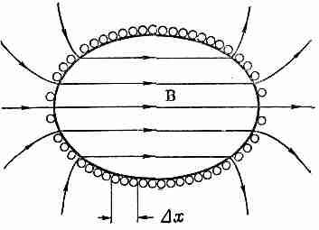
FIG. 29.4. Inside the ellipsoidal coil, which is current on any interval of the DX axis the same, a homogeneous field occurs.
But for this, the advantage has to be paid, because the method requires a large volume of a homogeneous magnetic field, and it is practically suitable for particles with small energy. If you remember, one of the methods for producing a homogeneous field is to wind the wire on the sphere so that the surface density of the current is proportional to the corner sinus. You can prove that the same is true for the ellipsoid of rotation. Therefore, very often such a spectrometer is made, simply wining ellipsoidal coils on a wooden or aluminum frame. The only thing that is required is that the current is at any interval of the axis Oh(FIG. 29.4) was the same.
§ 3. Electrostatic lens
Focusing particles has many applications. For example, in the television tube, electrons flying out from the cathode focus on the screen in a small spot. This is done in order to select the electrons of the same energy, but flying at different angles, and collect them into a small point. This task resembles focusing of light with lenses, so devices that perform such functions are also called lenses.
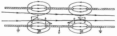
As an example of an electron lense, FIG. 29.5. This is an "electrostatic" lens, the action of which depends on the electric field between the two adjacent electrodes. Its work can be understood by following the fact that it does with a parallel parallel particle beam. Finding into the area A, the electrons experience force with the side component, which presses them to the axis. In the area of \u200b\u200bthe BEETS, it would seem, should be obtained equal in magnitude, but the opposite impulse on the sign, but it is not. By the time they reach the region b , energy will increase them somewhat, and therefore on the passage of the Boni region spend less time.
FIG. 29.5. Electrostatic lens.Showing power lines, i.e. QE vector lines.
The forces are the same, but the time of their action is less, therefore the impulse will be less. A full impulse of force when passing areas butand used to the axis, so as a result, the electrons are tightened to one common point. Leaving the high voltage area, the particles receive an added push towards the axis. In the area with strength directed from the axis, and in the region d - K.the axis, but in the second region of the particle remains longer, so that the full impulse is again directed towards the axis. For small distances from the axis, the full impulse of force throughout the lens is proportional to the distance from the axis (you understand why?), And this is just the basic condition necessary to ensure the focus of lenses of this type.
With the help of the same arguments, you can make sure that focus will be achieved in all cases where the potential in the middle of the electrode relative to two other or is positive or negative. Elektrostatic lenses of this type are commonly used in cathodechnic tubes and some electron microscopes.
§ 4. Magnetic lens
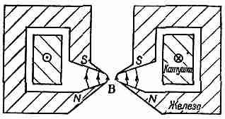
: There is another grade of lenses - they can often be found in electronic microscopes - these are magnetic lenses. Schematically, they are depicted in FIG. 29.6. Cylindrically symmetrical electromagnet with very sharp rings poles creates a very strong inhomogeneous magnetic field in a small area. It focuses electrons flying vertically through this area. The mechanism of focus is not difficult to understand; See an enlarged image of a region near pole tips in FIG. 29.7. You see two electrons butand B. , which leave the source S sby some angle in relation to the axis. As soon as electron butreaches the beginning of the field, the horizontal field component will dismiss it in the direction from you.It will acquire a side speed and, flying through a strong vertical field, will receive a pulse towards the axis. Side samethe movement is removed by the magnetic force when the electron leaves the field, so the final effect will be the impulse directed to the axis, plus the "rotation" relative to it.
FIG. 29.6. Magnetic lens.
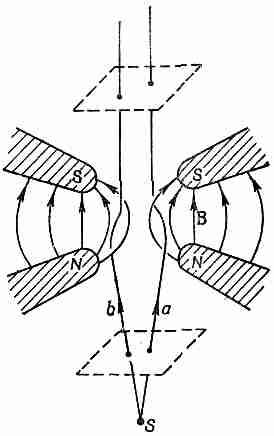
FIG. 29..7. Electron movement in magnetic lens.
There are the same forces on the particle, but in the opposite direction, so it also deviates towards the axis. The figure shows how the divergent electrons are collected in a parallel beam. The action of such a device is similar to the action of the lenses on the object in its focus. If now at the top put another such lens, it would focus the electrons again at one point and would have turned out the image of the source S.
§ 5. Electronic microscope
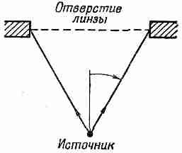
You know that the electronic microscope can "see" objects that are not available for the optical microscope. In ch. 30 (Vol. 3) We discussed the general limitations of any optical system caused by diffraction on the lens holes. If the lens opening is seen from the source at an angle of 2q (Fig. 29.8), then two neighboring points located near the source will be indistinguishable if the distance between them
FIG. 29.8. The microscope resolution is limited to the angular size of the lens relative to the focus.
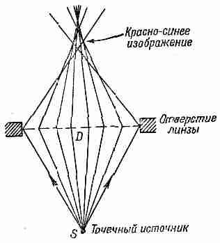
FIG. 29.9. Spherical aberration lenses.
in order of magnitude less
![]()
where l -light wavelength. For the best optical microscopes, the angle 6 is approaching the theoretical limit of 90 °, so B is approximately equal l., or about 5000 E.
The same limitations are applicable to the electronic microscope, but only the length of the waves in it, t, e. The wavelength of the electron electron with an energy of 50 kV is 0.05 E. If it were possible to use a lens with a hole of about 30 °, then we are capable We would distinguish objects in 1/5 A. Atoms in molecules are usually located at a distance of 1-2 e, therefore, then it would be possible to receive photos of molecules. Biology would be much easier; We could take a picture of the DNA structure. How it would be wonderful! After all, all today's research in molecular biology is attempts to determine the structure of complex organic molecules. If we were able to see them!
But unfortunately, the best permitting ability of electron microscopes is approaching only to 20 E. And all because so far no one has managed to build a lens with a big luminosity. All lenses suffer from "spherical aberration." This means that: rays going at a large angle to the axis, and the rays going close to it are focused at different points (Fig. 29.9). With the help of special technology, lenses are made for optical microscopes with negligible small spherical aberration, but it has not yet been possible to obtain an electron lens, devoid of spherical aberration. It can be shown that for any electrostatic or magnetic lenses of the types described by us, spherical aberration is inevitable. Along with the diffraction, aberration limits the resolution of electron microscopes by its modern value.
The restrictions on which we mentioned do not belong to electric and magnetic fields that do not have axial symmetry or not constant in time. It is possible that in
one day someone will come up with a new type of electronic lenses free from aberration inherent in simple electronic lenses. Then you can directly photograph atoms. It is possible that someday chemical compounds will be analyzed simply visual observation over the location of atoms, and not about the color of some kind of precipitate!
§ 6. Stabilizing accelerator fields
Magnetic fields are used in high-energy accelerators even in order to make the particle move along the desired trajectory. Such devices such as cyclotron and synchrotron accelerate a particle to high energies, forcing it to repeatedly pass through a strong electric field. And on its orbit, the magnetic field holds a particle.
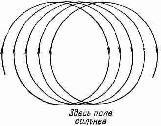
We have seen that the path of the particles in a homogeneous magnetic field passes along a circular orbit. But this is true only for the perfect magnetic field. And imagine that the field INin a large area, only approximately uniformly: in one part it is a little stronger than in another. If we start a particle with a pulse in such a field r,then she will fly around a circular orbit with a radius R \u003d P / QB.However, in the region of a stronger field, the radius of curvature will be slightly less. At the same time, the orbit will no longer be a closed circle, and the drift appears, similar to those shown in FIG. 29.10. If you want, we can assume that a small "error" in the field leads to a push, which shifts a particle to a new trajectory. In the accelerator, the particle makes millions of revolutions, so a kind of "radial focus" is necessary, which would hold the particle trajectories on close to the desired orbit.
Another difficulty associated with a homogeneous field is that the particles do not remain in the same plane. If they start moving at a small angle or a small angle is created by the inaccuracy of the field, then the particles go along the spiral path, which in the end will lead them either on the pole of the magnet or on the ceiling or floor of the vacuum chamber.
FIG. 29.10. Movement of particles in a slightly inhomogeneous field.
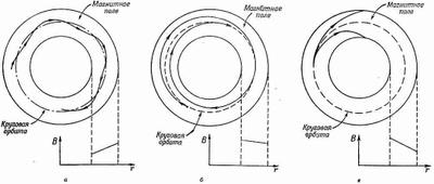
FIG. 29.11. Radial movement of particles in a magnetic field.
but -from a big positive "slope"; b -from a small negative "slope"; in -from a large negative "slope".
To avoid such a vertical drift, you need some devices; The magnetic field should provide both radial and "vertical" focus.
Immediately, you can guess that the radial focus provides a created magnetic field, which increases with increasing distance from the center of the designed path. Then, if the particle goes to a larger radius, it will be in a stronger field that will return it back to the desired orbit. If it goes to a smaller radius, then "bending" will be less and it will return back to the desired radius. If the particle suddenly began to move at an angle to an ideal orbit, it will start oscillating relative to it (FIG. 29.And, but)and the radial focus will hold the particle near the circular path.
Actually radial focus occurs even at opposite"Tilt". This may occur in cases where the radius of the curvature of the trajectory increases no faster than the distance of the particles from the center of the field. Particle orbits will be similar to those shown in FIG. 29.11.6. But if the gradient of the field is too large, the particles will not return to the desired radius, and will be on the helix to leave the field either inside or outward (Fig. 29.11, in).
![]()
"Tilt" fields we usually describe a "relative gradient", or index of field N.
The guide field creates radial focus, if the relative gradient is more -1.
The radial gradient of the field will also lead to verticalforces acting on a particle. Suppose we have a field that near the center of the orbit is stronger, and the outside is weaker. The vertical cross-section of the magnet at a right angle to orbit may have such a look as shown in FIG. 29.12. (And the protons fly to us from the page.) If we need the field to be stronger to the left and weaker to the right, then magnetic power lines should be twisted as shown in the figure. The fact that it should be so can be seen from the law of equality zero circulation in empty
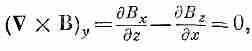
trank. If you select the coordinate system shown in the figure, then
![]()
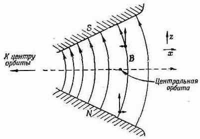
FIG. 29.12. Vertically focusing field.
Cross-sectional view perpendicular to orbit.
Since we assume that dv z. / dh.negatively, it should be equal to him and negative dv h. / dz. If a"Nominal" plane of the orbits is the plane of symmetry, where IN h. =0, that radial component IN h. It will be negative above the plane and positive under it. In this case, the lines must be twisted as shown in the figure.
This field must have vertically focusing properties. Imagine a proton flying more or less parallel to the central orbit, but above it. The horizontal component in will act on a proton with a force directional. If the proton is below the central orbit, the force will change its direction. Thus, an effective "restoring force" arises, directed towards the center of the orbit. From our reasoning it turns out that, subject to reduction verticalthe fields with increasing radius should be vertical focus. However, if the gradient of the field is positive, then the "vertical defocus" occurs. Thus, for vertical focusing, the field index is not less than zero. Above we found that for radial focusing, the value of becoming more -1. The combination of these two conditions requires for hold of particles in stable orbits to
In cyclotrons, N value is usually used , approximately equal to zero, and in betatrons and synchrotrons a typical value is n \u003d -0.6.
§ 7. Focusing with an alternating gradient
So small values \u200b\u200bare pretty "weak" focus. It is clear that much greater radial focus could be obtained for a large positive gradient. (N \u003e\u003e 1),but at the same time, the vertical forces will be strongly defocused. Similarly, a large negative tilt (NB and the focusing effect.
To explain how it works such focuswe first analyze the action of a quadrupole lens, which is arranged on the same principle. Imagine that the magnetic field shown in FIG. 29.12, a homogeneous negative magnetic field was added, which is chosen so that the field in orbit is zero. The resulting field with low offsets from the neutral point will resemble the shown in FIG. 29.13. Such a four-pole magnet is called a quadrupole lens. A positive particle that enters (from the reader) to the right or to the left of the center, is again drawn into the center. If the particle comes from above or from the bottom from the center, then it pushes outout of him. This is a horizontal focusing lens. If you reach a horizontal gradient now, which can be done by the variety of all poles to the opposite, then the sign of all forces will change to the opposite and we get a vertically focusing lens (Fig. 29.14). The field strength in such lenses, and consequently, the focusing force increase linearly by removing the lens from the axis.
Imagine now that we put two such lenses in a row. If the particle is included with some horizontal displacement relative to the axis (Fig. 29.15, but),it will deviate towards the axis of the first lens. When it is suitable for the second lenses, it turns out to be closer to the axis, where the ejecting force is less, so the deviation from the axis will be less.
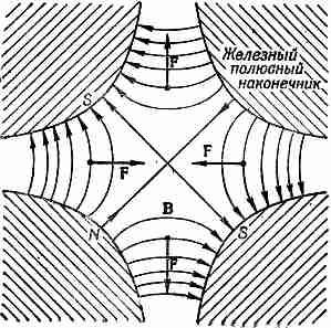
FIG. 29.13. Horizontally focusing quadrupole lens.
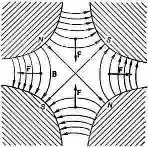
FIG. 29.14. Vertically focusing quadrupole lens.
As a result, there will be a slope to the axis, i.e. averagetheir action will be horizontal focusing. On the other hand, if we take a particle that deviates from the axis in the vertical direction, the path will be like that, as shown in FIG. 29.15, b.The particle is first deflected from the axis, andthen he enters the second lens with a large displacement, experiencing the effect of greater strength, resulting in deviating to the axis. In general, the effect will be focusing again. Thus, the action of a pair of quadrupole lenses acting independently in horizontal and vertical directions is very similar to the action of an optical lens. Quadrupole lenses are used to form a beam of particles and control over it in accuracy as well as optical lenses are used for a light beam.
It should be emphasized that the variable-gradient system does not always lead to focus. If the gradient is too large (compared with the particle pulse or with a distance between the lenses), then the resulting action will be defocusing. You will understand how it turns out if you imagine that the space between the two lenses in FIG. 29.15 increased three or four times.
And now back to the synchrotron guide magnet. It can be considered that it consists of an alternating sequence of "positive" and "negative" lenses with a homogeneous field superimposed on top. The homogeneous field is used to hold particles on average on the horizontal circle (it does not affect the vertical movement), and the lenses variable act on any particle that strives to get rid of the way, pushing it all the time to the central orbit (on average).
There is a very good mechanical analog that demonstrates how the variable "focusing and defocusing" force can result in the "focusing" effect. Imagine a mechanical "pendulum" consisting of a solid rod with a loader suspended on the axis, which, with the help of a crank associated with the engine, can quickly
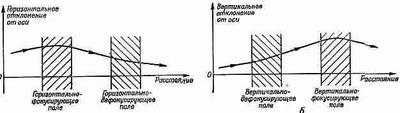
FIG. 29.15. Horizontal and vertical focusing by a pair of quadrupole lenses.
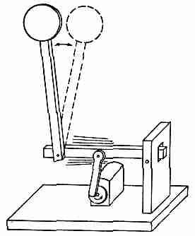
FIG. 29.16. The pendulum with an oscillating axis has a stable position with the weights located at the top.
rash up and down. This pendulum has twoequilibrium positions. In addition to the normal position, when the pendulum hangs down, he still has an even position of equilibrium when he sticks out up, - Georgic is located overpoint of support (Fig. 29.16).
Simple arguments show that the vertical movement of the rod is equivalent to the focusing force variable. When the rod accelerates down, the Georgian seeks to move towards the vertical, as shown in FIG. 29.17, and when the Georgic is accelerated up, everything happens in the reverse order. But despite the fact that the power changes its direction all the time, on average it acts to the vertical. Thus, the pendulum will swing there and here near the neutral position, which is exactly opposite to normal.
There is, of course, a simpler way to keep the pendulum "upside down" - for example balancehis finger. But try it to keep so two independentpendulist on one finger.Or even one, but with closed eyes. Balancing means making small amendments to what is wrong. And if several parameters are simultaneously incorrect, then balancing is impossible in most cases. However, in the synchrotron in orbit, billions of particles are moving at the same time, each of which has its own "error", and yet the focusing method described by us acts immediately to all these particles.
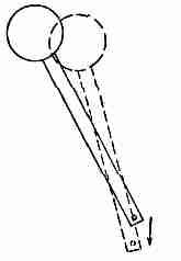
FIG. 29.17. Acceleration of the axis of the pendulum down
leads to the movement of it towards the vertical.
§ 8. Movement in crossed electrical and magnetic fields
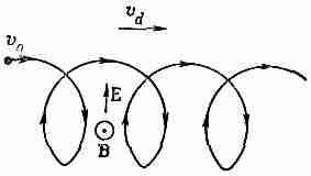
So far, we talked about particles that are only electrically or only in a magnetic field. But there are interesting effects that occur with the simultaneous action of both fields. Let us have a homogeneous magnetic field B and directed to it at a right angle electrical field E. Then the particles flying perpendicular to the field in will move along the curve similar to those shown in FIG. 29.18. (It flatcurve, A. notspiral.) Qualitatively this movement understand it is not difficult. If the particle (which we consider positive) moves in the direction of the field e, then it gains speed, and the magnetic field bends it less. And when the particle moves against the field e, it loses the speed and gradually more and more bended to the magnetic field. As a result, the drift is obtained in the direction (EX).
We can show that such a movement is essentially a superposition of uniform movement at speeds v. d. \u003d E / Band circular, i.e. in FIG. 29.18 shows simply cycloid. Imagine an observer who moves to the right at a constant speed. In its reference system, our magnetic field is converted to a new magnetic field. a pluselectric field downward. If its speed is chosen so that the total electric field is equal to zero, the observer will see the electron moving around the circle. Thus, movement that wewe see, it will be a circular motion plus transfer with the drift speed v. d. \u003d E / B.The movement of electrons in crossed electrical and magnetic fields underlies magnetonov, i.e. oscillators used in the generation of microwave radiation.
There are still many other interesting examples of the movement of particles in electrical and magnetic fields, such as the orbits of electrons or protons trapped in radiation belts in the upper stratosphere, but, unfortunately, we do not have enough time to engage in these issues now.
FIG. 29.18. The path of the particles in the crossed electrical and magnetic fields.
qV x in always acts at right angles to the direction of movement, so that the DP / DT derivative is perpendicular to P and is equal to the value of VP / R, where R is the circle radius, i.e.
46. Traffic electric charge in a constant and homogeneous magnetic field.
47. Electric charge movement in mutually perpendicular electrical and magnetic fields.
48. Magnetic field in substance. Magnetic permeability of the medium. Diagrams and ferromagnetics. Magnetic field strength.
49. Phenomenon electromagnetic induction. The law of electromagnetic induction. Lenza rule.
The phenomenon of electromagnetic induction was opened in 1831. Michael Faraday (Faraday M., 1791-1867), which established that in any closed conductive circuit when changing the magnetic induction stream through the surface bounded by this circuit, an electric current occurs, called it induction. The value of the induction current does not depend on the method that the change in the flow of magnetic induction is caused, but is determined by the speed of its change, that is, the value. When the sign changes, the direction of the induction current is also changing.
E.H.Lenz (1804-1865) set the rule according to which the induction current in the circuit is always directed in such a way that the magnetic flux created by it through the surface bounded by the contour, tends to prevent this change in the magnetic flux that caused the appearance of this current.
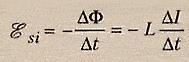
To create a current in a closed circuit, it is necessary to have an electromotive force. The phenomenon of electromagnetic induction indicates that when changing the magnetic flux in the circuit arises EMF induction εi, the size and direction of which depend on the rate of change of this stream. After analyzing the results of Faraday's experiments, Maxwell (Maxwell J., 1831-1879) gave the main law of electromagnetic induction the following modern appearance:
The sign "-" in this formula corresponds to the ruler of Lenz and means that the direction of EMF εi and the direction of changes in the flow of magnetic induction are interconnected by the rule of the left screw. We emphasize that speaking of "direction" scalar quantities εi and, you need to understand this term in the same sense, which is invested, for example, in the concept of current direction.
The flow of the magnetic field induction through the surface S, the limited outline circuit is determined by the expression:
The unit of measurement of the magnetic induction flow in C is Weber: 1B \u003d T ∙ M2. With the rate of change of induction flow, equal to 1B / s, an EDC is induced in the circuit equal to 1B.
Substituting the expression for the Faraday law, we will have:
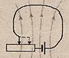
It can be seen that the appearance of an induction EMF and, accordingly, induction current in a conductive circuit can be caused by each of two reasons: 1) in a fixed circuit - due to changes in the time of induction of the magnetic field (Fig.14.1); 2) in a moving conductor - due to the intersection of the power lines of the magnetic field (Fig.14.2).
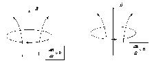
Fig.14.1. The occurrence of induction current in a fixed closed circuit.
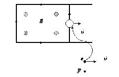
Fig.14.2. The occurrence of induction current in a moving conductor.
50. Self-induction. EMF ( Electromotive force) self-induction. Inductance.
Self-induction - the emergence of EMF induction in a closed conductive circuit when the current changes through the contour.
When the current changes, the magnetic flux through the surface limited to this circuit is changed in the circuit. The change in this magnetic flux, by virtue of the law of electromagnetic induction, leads to an initiation in this circuit inductive EMF.
This phenomenon is called self-induction. (The concept is known to the concept of mutually induction, being as if its private case).
The direction of self-induccous EMF always turns out to be such that, with an increase in current in the EMF chain, self-induction prevents this increase (directed against the current), and when decreasing current - descending (coated with current). This property of self-induction EMF is similar to the power of inertia.
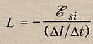
The magnitude of self-induction EMF is proportional to the speed of change of current:
The proportionality coefficient is called self-induction coefficient or contour inductance (coil).
Self-induction
Each conductor for which El.tok flows is in its own magnetic field.
When the current change in the conductor changes M. POLE, i.e. The magnetic flux created by this current changes. The change in the magnetic flux leads in the occurrence of vortex email and in the circuit appears induction.
![]()
This phenomenon is called self-induction.
Self-induction - the phenomenon of the occurrence of EMF induction in an email fall as a result of a change in the current force.
The emerging EMF is called EMF self-induction
Manifestation of the phenomenon of self-induction
Circuit chain
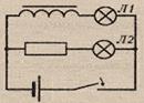
When closing in the email, the current increases, which causes an increase in magnetic flux in the coil, a vortex email appears, directed against the current, i.e. In the coil, self-induction emfs occurs, which prevents the increase in the current in the chain (the vortex field slows down the electrons).
As a result, L1 lights up later than L2.
Blurring chain
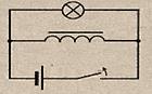
When operating an email deck decreases, a decrease in M.Potok in the coil arises, the vortex email appears, directed as the current (striving to preserve the former current strength), i.e. In the coil there is a self-induction EMF, which maintains the current in the chain.
As a result, when it turns off brightly flashes.
in the electrical engineering, the self-induction phenomenon manifests itself when the chain is closed (email increases gradually) and when the circuit is blurred (email does not disappear).
INDUCTANCE
What does emd self-induction depend on?
El .To creates its own magnetic field. Magnetic flow through the contour is proportional to the induction of the magnetic field (F ~ B), the induction is proportional to the current power in the conductor
(B ~ i), therefore, the magnetic flow is proportional to the strength of the current (F ~ I).
EMF of self-induction depends on the rate of change of current in the email, from the properties of the conductor
(sizes and shapes) and on the relative magnetic permeability of the medium in which the conductor is located.
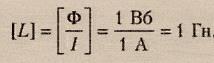
The physical value showing the dependence of self-induction EMF from the size and shape of the conductor and on the medium in which the conductor is called the self-induction coefficient or inductance.
Inductance - Phys. The value is numerically equal to self-induction EMF arising in the circuit when the current is changed by 1 per 1 second.
![]()
where F is a magnetic flow through the contour, I is the current strength in the circuit.
Units of inductance in the SI system:
The inductance of the coil depends on:
numbers of turns, sizes and shapes of the coil and from relative magnetic permeability of the medium
(Candle is possible).
EMF self-induction
EMF of self-induction prevents the increase in current force when the circuit is turned on and decreasing the current for the circuit of the chain.
51. Energy and density of the magnetic field.
The conductor, with the electric current flowing along it, is always surrounded by a magnetic field, and the magnetic field disappears and appears along with the disappearance and appearance of the current. Magnetic field, like electrical, is a carrier of energy. It is logical to assume that the magnetic field energy coincides with the work spent current to create this field.
Consider the circuit of the inductance L, according to which the current I flows. The magnetic flux F \u003d Li is connected with this circuit, since the inductance of the contour is unchanged, then when the current changes on the Di, the magnetic flux changes to DF \u003d LDI. But to change the magnetic flux by the value of DF, you should make the operation of DA \u003d Idf \u003d LIDI. Then work on the creation of a magnetic flux F is equal
![]()
So, the energy of the magnetic field, which is associated with the contour,
The magnetic field energy can be considered as a function of values \u200b\u200bthat characterize this field in the surrounding space. To do this, consider a special case - a homogeneous magnetic field inside a long solenoid. Substituting in formula (1) the solenoid inductance formula, we will find
![]()
Since I \u003d BL / (μ0μN) and B \u003d μ0μH, then
![]() (2)
(2)
where Sl \u003d V is the volume of the solenoid.
The magnetic field inside the solenoid is uniformly and focused inside it, so the energy (2) is concluded in the volume of solenoid and has a homogeneous distribution with a constant volumetric density with it.
Formula (3) for bulk energy density of the magnetic field is similar to expression for bulk energy density electrostatic fieldwith the difference that electrical values Replaced with magnetic. Formula (3) was shown for a homogeneous field, but it is true for inhomogeneous fields. Formula (3) is valid only for media for which a linear dependence in from H, i.e. It applies only to para- and diamagnets.
52. System Maxwell Equation for electromagnetic field. Shift current.
Maxwell Equations - System differential equationsdescribing the electromagnetic field and its connection with electrical charges and currents in vacuum and solid media. Together with the expression for the power of Lorentz form full system Equations of classical electrodynamics. The equations formulated by James Clerk Maxwell on the basis of experimental results accumulated by the middle of the 19th century, played a key role in the development of the aspects of theoretical physics and had a strong, often decisive, influence not only on all areas of physics directly related to electromagnetism, but also for many subsequently related Fundamental theories, the subject of which did not boost to electromagnetism (one of the brightest examples here can serve special theory Relativity
The Maxwell Theory is based on four equations considered above:
1. The electric field can be both potential (EQ) and vortex (EB), therefore the intensity of the total field E \u003d EQ + EB. Since the circulation of the EQ vector is zero (see (137.3)), and the circulation of the EB vector is determined by the expression (137.2), the circulation of the tension of the total field
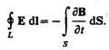
This equation shows that the sources of the electric field can not only be electrical charges, but also changing magnetic fields.
2. Generalized vector circulation theorem
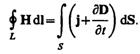
This equation shows that magnetic fields can be excited by either moving charges (electrical currents) or by variable electric fields.
3. The Gaussian Theorem for Field D
If the charge is distributed inside the closed surface continuously with the bulk density R, then formula (139.1) is recorded as
![]()
4. Gaussian theorem for field in
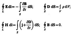
So, the complete system of Maxwell equations in the integral form:
The values \u200b\u200bincluded in the Maxwell equations are not independent and between them there is the following connection (isotropic non-ferromic and non-ferromagnetic environments):
where E0 and M0 are the electrical and magnetic constant, E and M, respectively, respectively, dielectric and magnetic permeability, G is the specific conductivity of the substance.
Of the Maxwell equations, it follows that either electrical charges or magnetic fields change in time can be sources, and magnetic fields can be excited by either moving electrical charges (electrical currents) or by variable electric fields. Maxwell equations are not symmetric about electric and magnetic fields. This is due to the fact that in nature there are electrical charges, but there are no charges of magnetic.
For stationary fields (E \u003d const and B \u003d Const) Maxwell equations will take a view
those. Sources of the electric field in this case are only electrical charges, sources of magnetic - only conductivity currents. In this case, electrical and magnetic fields are independent of each other, which allows to study separately constant electrical and magnetic fields.
Taking advantage of the Stokes and Gauss theorems known from the vector analysis
you can present the complete system of Maxwell equation in differential form (characterizing the field at each point of space):
If charges and currents are distributed in space continuously, both forms of Maxwell equations are integral and differential - equivalent. However, if there are surfaces of the break - the surfaces on which the properties of the medium or fields are scanned, then the integral form of equations is more general.
Maxwell's equations in differential form assume that all values \u200b\u200bin space and time change continuously. In order to achieve the mathematical equivalence of both forms of Maxwell equations, the differential form is complemented by the boundary conditions, which should satisfy the electromagnetic field at the border of the section of two environments. Integral form Maxwell equations contain these conditions. They were reviewed earlier:
(The first and last equation correspond to cases when there are no free charges on the border of the section, no conductivity currents).
Maxwell equations are the most common equations for electrical and magnetic fields in resting media. They play in the teaching about electromagnetism the same role as Newton's laws in mechanics. From the Maxwell equations it follows that the alternating magnetic field is always associated with an electric field generated by it, and the variable electric field is always associated with the magnetic generated by it, i.e., the electric and magnetic fields are inextricably linked with each other - they form a single electromagnetic field.
Maxwell's theory, being a generalization of the basic laws of electrical and magnetic phenomena, not only was able to explain the already known experimental facts, which is also an important consequence, but also predicted new phenomena. One of the important conclusions of this theory was the existence of a magnetic field of displacement currents, which allowed Maxwell to predict the existence of electromagnetic waves - an alternating electromagnetic field propagating in space with a deadline. In the future, it was proved that the rate of propagation of the free electromagnetic field (not related to charges and currents) in vacuo is equal to the speed of light C \u003d 3 × 10⁸ m / s. This conclusion and theoretical study of the properties of electromagnetic waves led Maxwell to the creation electromagnetic theory Lights according to which the light is also electromagnetic waves. Electromagnetic waves on experience were obtained by German physicist. Herz (1857-1894), which have proven that the laws of their excitation and distribution are fully described by the Maxwell equations. Thus, Maxwell's theory was experimentally confirmed.
Shift current. When building the theory of the electromagnetic field, J. K. Maxwell pushed the hypothesis (subsequently confirmed on the experience) that the magnetic field is created not only by the movement of charges (conduction current, or simply current), but also by any change in the time of the electric field. Value equal to the rate of change in time (T) electric induction D (more precisely, the amount
(D / T) / 4P), Maxwell called the shift current. The vortex magnetic field is determined full current J \u003d JPR + (D / T) / 4P, where JPR is the density of conduction current. The bias current creates a magnetic field by the same law as the conductivity current, and the name "Current" for the value (D / T) / 4P is associated with it.
If the alternating magnetic field creates the electric field, it is reasonable to assume the existence and reverse process: the changing electric field generates the magnetic field. Such a phenomenon really exists and wears not quite the usual name of the shift current
Electric charge. His discreteness. The law of conservation of an electric charge. Cut law in vector and scalar form.
Electric charge - this is physical quantity, characterizing the property of particles or bodies to join electromagnetic power interactions. Electric charge is usually denoted by letters Q or Q. There are two kinds of electric charges, conditionally mentioned positive and negative. Charges can be transmitted (for example, with direct contact) from one body to another. Unlike body weight, an electrical charge is not an integral characteristic of this body. The same body in different conditions May have a different charge. The charges of the same name are repelled, the variepetes are attracted. Electron and proton are respectively carriers of elementary negative and positive charges. The unit of electric charge is a pendant (CL) - an electrical charge passing through a cross-section of the conductor at a current of 1 and during 1 s.
Electric charge discreteen, i.e. the charge of any body is a variety of elementary electric charge E ().
The law of saving charge: The algebraic amount of electrical charges of any closed system (a system that does not exchange charges with external bodies) remains unchanged: Q1 + Q2 + Q3 + ... + Qn \u003d Const.
The law of Kulon. : The strength of the interaction between two point electrical charges is proportional to the values \u200b\u200bof these charges and is inversely proportional to the square square between them.
![]() (in a scalar form)
(in a scalar form)
Where F is the culon force, Q1 and Q2 - the electric charge of the body, R is the distance between charges, e0 \u003d 8.85 * 10 ^ (- 12) - the electrical constant, the E-dielectric permeability of the medium, k \u003d 9 * 10 ^ 9 - Proportionality coefficient.
To perform the law of the coulon, it is necessary 3 conditions:
1 condition: the point of charges - that is, the distance between the charged bodies is much more than their sizes
2 Condition: Stated immobility. Otherwise, additional effects come into force: the magnetic field of the moving charge and the corresponding additional force of Lorentz, acting on another moving charge
3 Condition: Interaction of charges in vacuum
In vector The law is written as follows:
![]()
Where - the force with which the charge 1 is valid for charge 2; Q1, Q2 - the value of charges; - radius vector (vector directed from charge 1 to charge 2, and equal, module, distance between charges -); k - proportionality coefficient.
Electrostatic field strength. Expression for the tension of the electrostatic field point charge in vector and scalar form. Electric field in vacuo and substance. The dielectric constant.
The tension of the electrostatic field is vector silence characteristic Fields and numerically equal to the power with which the field acts on a single test charge made at this field:
The unit of tension is 1 N / CL - it is the strength of such an electrostatic field, which for charge in 1 CL acts with force in 1 N. Tension is also expressed in per / m.
As follows from the formula and law of the coulon, the intensity of the spot charge field in vacuum
![]() or
or ![]()
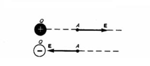
The direction of the vector E coincides with the direction of force, which acts on a positive charge. If the field is created by a positive charge, the vector E is directed along the radius-vector from charge in external space (pushing the trial positive charge); If the field is created negative charge, the vector E is directed to the charge.
So Tension is the power characteristic of the electrostatic field.
For graphic image The electrostatic field use vector strength lines ( power lines). In the thickness of the power lines, one can judge the magnitude of tension.
If the field is created by the charge system, the resulting force acting on the test charge made at this field is equal to the geometric sum of the forces acting on the test charge from each point charge separately. Therefore, the tension at this point of the field is equal to:
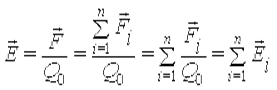
This ratio expresses principle of superposition fields: The tension of the resulting field created by the charge system is equal to the geometric sum of the field strengths created at this point by each charge separately.
Electricity Vacuum can be created by the ordered movement of any charged particles (electrons, ions).
The dielectric constant - The value characterizing the dielectric properties of the medium is its reaction to the electric field.
In most dielectrics with not very strong fields the dielectric constant does not depend on the field E. in the strengths electric fields (comparable with intra-nuclear fields), and in some dielectrics in conventional fields dependency D from E is nonlinear. The dielectric constant shows how many times the strength of the interaction F between electric charges in this medium is less than their strength of the FO in vacuo
The relative dielectric permeability of the substance can be determined by comparing the test capacitor capacity with this dielectric (CX) and the capacitance of the same capacitor in vacuum (CO):
![]()
Electrostatic field strength. Movement of charged particles in a uniform electric field.
In a homogeneous electric field, the force acting on the charged particle is constant both in magnitude and in the direction. Therefore, the movement of such a particle is completely similar to the body movement in the field of gravity of the Earth without taking into account air resistance. The trajectory of the particle in this case is flat, lies in the plane containing the veneer vectors of the particle and electric field strength