Determination of voltage and tension potential. Potential difference, charge energy in the electric field. Potential

We now turn to spherical (point) charge. Above shows that tension electric fieldcreated uniformly distributed in the sphere Q., does not depend on the radius of the sphere. Imagine that at some distance r. From the center of the sphere is a trial charge q.. The intensity of the field at the point where the charge is

The figure shows a graph of the dependence of the force of electrostatic interaction between the point charges from the distance between them. To find the work of the electric field when moving the test charge q. With distance r. up to distance R., disarm this gap dots r. 1 , r. 2 ,..., r. P on equal segments. The average force acting on the charge q. within the segment [ rR 1], equal

The work of this force on this site:

Similar expressions for work will be obtained for all other sections. Therefore, full work:

The same terms are destroyed with opposite signs, and we finally get:

- work fields above charge

- Potential difference

Now, to find the potential of the point of the field regarding infinity, ascertain R. To infinity and finally get:

So, the potential of the field point charge Inversely proportional to the distance to charge.

24. Potential charge energy in the charge system field. The principle of superposition for potentials. Superposition principle for potentials

Any as an acclacent electrostatic field can be represented as superposition of spot charges. Each such field in the selected point has a certain potential. Since the potential is a scalar value, the resulting potential of the field of all point charges is the algebraic amount of potentials 1, 2, 3, ... fields of individual charges: \u003d 1 + 2 + 3 + ... This ratio is a direct consequence of the principle of superposition of electric fields.

Potential charge energy in the electric field. Continue comparing the gravitational interaction of bodies and electrostatic interaction of charges. Body mass m.in the gravity of the earth has potential energy. The work of gravity is equal to the change in the potential energy taken with the opposite sign:

A \u003d -(W. p2. - W. p1) = mGH.

(Here and then we will denote the energy of the letter W..) In the same way as the body mass m. In the field of gravity, has potential energy, proportional mass of the body, electric charge in the electrostatic field has potential energy W. p proportional to charge q.. Work of the power of the electrostatic field BUT equal to changing the potential energy of charge in electric fieldtaken with the opposite sign:

A \u003d -(W. p2. - W. p1) . (40.1)

25. Potential difference. Equipotential surfaces

Equipotential surface - Surface, each point of which has the same potential.

As follows from the connection of work and potentials:

when transferring the charge along the equipotential surfaces, the electric field does not perform, since.

Work with nonzero power is zero only if the strength vector is perpendicular to the movement vector. It follows from this that the lines of tension are perpendicular to the equipotential surfaces. Examples of equipotential surfaces serve as sphere for a point charge field and parallel planes for homogeneous fields (Fig. 3).

Potential difference (voltage)between the two points is equal to the function of the field when the charge is moved from the starting point to the final to the module of this charge: U. \u003d φ 1 - φ 2 \u003d -Δφ \u003d A / Q, A \u003d - (W p2 - W p1) \u003d -q (φ 2 - φ 1) \u003d -qδφ

The potential difference is measured in volts (B \u003d J / CL) communication between tension electrostatic field and potential difference: e x. = Δφ / Δ x. The voltage of the electrostatic field is directed toward the decrease in the potential. Measured in Volts divided by meters (in / m)

In the previous paragraph, we discussed the basic characteristics of the electric field - its tension. As it follows from the very definition is a power characteristic, which means the vector. In some cases, more convenient are scalar characteristicswhich it turns out to be also introduced for the electrostatic field - the difference of potentials and potential. At the same time, we will rely on the important fundamental property of the forces acting on the charge in the electrostatic field - their conservatism.

Recall that conservatives are called forces whose work does not depend on the form of the trajectory of the body movement. The work of such forces is determined by the coordinates of the initial and endpoint movement points. Relying on our knowledge of the properties of its power characteristics of the electrostatic field created by an arbitrary system of charges, it would be possible to carry out a detailed proof of equality of work when the charge moves between any two points. But we will slightly reduce this procedure, remembering the theorem "On the conservatism of the central forces", we have proven in the mechanics section.

The fixed point charge is the source of the "field of the central forces" - this directly follows from the formulation of the basic law of electrostatics - the law of Culon. From the principle of superposition of electric fields it follows that work when moving a trial charge in the field of any system rest The charges are an algebraic amount of work in the field of each of the charges separately. So, the field of such forces ("Coulomb forces" *) is also a field of conservative forces. This was required to prove.

Thus, the operation of the power of the electrostatic field **) to move the point (trial) charge between two points characterizes this field. But it depends on the size of the test charge q. 0. This is what experiences experience, but this is understandable and, on the basis of our knowledge of the "Coulomb" forces. After all, they are proportional to the charge Q. 0 At each point of the trajectory 1®2 (based on the Culon law), and the work is proportional to force. To characterize the field and only the field can be divided into work on the value of the trial charge. What will happen and is the "potential difference". We give the definition of this important concept:

(OPR .) Potential difference between points of the electrostatic field 1 and 2 are called attitude work Fields to move a test charge from point1 exactly2 To the magnitude of this charge :

. (3.1)

In the system SI, the unit of measurement of potential difference is 1 volt (1 V \u003d 1 J / CL). If we learn how to determine the difference in potentials J. 1 –j. 2 for the field of the system of resting charges (theoretically or experimentally), this will allow you to find the work of the field to move any pottle Charge q. In this field:

. (3.2)

Thus, the potential difference is energy characteristic The electric field, since it is connected directly to the concept of work.

In the mechanics, we introduced for conservative forces (now we, say: "fields of conservative forces") the concept of "potential energy". At the same time, we were guided by the following principle: "The work of the forces of the field is equal to the decrease of potential energy." We formalize this principle in analytical record:

Here u 1 and u 2 are potential energy in the "initial" ("1") and "final" ("2") states of the system, respectively. In the case under discussion, the field of fixed charges system is the energy of a point charge q.in the position "1" (with coordinates ( x. 1 ,y. 1 ,z. 1)) and the position "2" (with coordinates ( x. 2 ,y. 2 ,z. 2)) electrostatic field. Those. The potential charge energy in this field is the scalar function of the coordinates of the points of the field U \u003d U ( x.,y.,z.) (or ). Comparing (3.2) and (3.3), we see - it is convenient to assume that the potential difference is the difference of the values \u200b\u200bof another scalar function of the coordinates of the field points j.(x, Y, Z). It is associated with the function U ( x.,y.,z.) (potential energy) simple ratio: u ( x.,y.,z.) = q.× j.(x, Y, Z). Or, since

it is said that it is "numerically equal to the potential energy of a single positive charge" at this point point. And called this value j."Potential" of this point of the electrostatic field.

The most important thing is how to find this feature for the field of a particular charge system? What is the procedure for action?

First of all, you have to agree on normalization conditions *): You need to choose a point R 0, in which the potential of the test charges will assume equal to zero. Most often, such a point is chosen "infinitely" remote, where there is no field **). To do this, you need to find the "specific" work of the field -T.E. Work attributed to the value of the portable test charge (or, as often spoke, "to move a single positive" charge) from this point of the field R(x.,y.,z.) to the ignition point R 0. In analytical form it definition The potential can be written as:

(ORD. ) j R.(x.,y.,z.) = . (3.5)

Would we not express the newly introduced values \u200b\u200b- the potential difference and potential through the power characteristic, which we have learned to count on the specified location of charges in space? Sure you may. We write the chain well-understandable equals:

Drinking the last equality again

. (3.6)

It gives a "recipe" search for the potential difference according to the known level of tension. Similarly for potential:

And finally for the potential of an arbitrary point of the field R with coordinates ( x.,y.,z.):

. (3.7)

· Potential Pattern Point Charge

Relying on the procedure for calculating the potential, we obtain an expression for the case of a point charge field. This is very important for further calculations of the potential of the system of the system arbitrarily located in the space of charges.

2. Selection of the trajectory. Let an arbitrary point R(x.,y.,z.) is at a distance r.from the source charge. Since the result does not depend on the form of the trajectory to calculate the curvilinear integral of the form (3.7), select the simplest radially directed direct line of this point along the power line and "flowing into infinity."

3. Payment. In accordance with the determination of the potential, we will perform the calculation of the "specific" work of the field created by a point charge q.by transferring a test charge along the selected trajectory. The following chain of equalities, hope it looks like "transparent". However, we will give it a minimum comment. First of all, we note that due to our choice of the trajectory in the form of a radially directed from the charge of the beam, you can designate E L.and dL(arbitrary curve " L.") change to E R. and dr.(polar axis " r."). Moreover, since the vector is directed radially, for any small movement along the trajectory, the projection of the voltage vector is simply the module of this vector E.(r.). As a result, we can make an important step in our calculation - to make the transition from the curvilinear integral to the usual definite:

.*)

Now after substituting the expression for the intensity module of a point charge (3.5), we remain only mathematical "routine":

We repel the result again, adding it by taking into account the possible presence of a gaseous or liquid homogeneous dielectric medium with permeability e.Filling out all surrounding point charge Space:

. (3.8)

Potential field of point charge, as we see, decreases with distance by law 1 / r..

· Equipotential surfaces

When discussing silence characteristics The electrostatic field we were convinced of the fruitfulness of the concept silest lines (voltage lines). For the energy characteristics of the field - potential - it is also useful to introduce an additional illustrative characteristic - the system of "equipotential surfaces". From the very name is clear ("Equiva" means "equal"), which is the surfaces of constant potential, which characterize the ability of the field forces to make work when the charge is moving. Along such surfaces, the work is obviously not performed at all. It is maximal in the directions for which the maximum density (density) of the location of the equipotential surfaces. In these places the maximum and voltage of the field. It is easy to figure out what the mutual orientation of power lines and equipotential surfaces in the places of their intersections are: they are mutually perpendicular. After all, with any small move along equipotential surface elementary work equal to zero, and this is possible only if it is zero by the tangent component of the voltage vector, i.e. It is directed strictly by normal to the surface. Below we give a chain of the corresponding words, we hope quite obvious equalities:

Together with Fig. 3. ... They prove, in essence, the already formulated statement: power lines crossed (or "fit to ...") equipotential surfaces at right angles !

We present the picture of the equipotential surfaces (and the power lines too) for some simplest already well-known cases of the electrostatic field: but) point of point charge; b.) The field of two characters in the module of the varied point charges; in) The field between two variestly charged with plane-parallel large (compared to the distance between them) plates - see Fig. 3.1.

The potential of the electric field is the ratio of potential energy to the charging. As you know the electric field is potential. Consequently, any body in this field has potential energy. Any work that will be accomplished by the field will occur due to a decrease in potential energy.

Formula 1 - Potential

Electric field potential is the energy characteristics of the field. It represents the work that needs to be made against the electric field forces in order to move a single positive point charge on infinity at this field.

The potential of the electric field in volts is measured.

If the field is created by several charges that are arranged in an arbitrary order. The potential at this point of such a field will be an algebraic amount of all potentials that are individually created by charges. This is the so-called superposition principle.

Formula 2 - the total potential of different charges

Suppose that in the electrical field the charge is moved from the "A" point to the point "B". Work is performed against the power of the electric field. Accordingly, the potentials at these points will differ.

Formula 3 - Work in the electric field

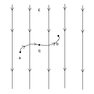
Figure 1 - The movement of charge in the electric field

The potential difference between two field points will be equal to one volt, if to move the charge into one pendant between them, it is necessary to work in one joule.

If the charges have the same signs, the potential energy of the interaction between them will be positive. In this case, charges are repelled from each other.

For multi-charged charges, the energy of the interaction will be negative. The charges in this case will be attracted to each other.

Topic 3. The potential and operation of the electrostatic field. Tension connection with potential

3.4. Dipole in the electric field

3.5. The relationship between the tension and the potential of the electrostatic field

3.6. Power lines and equipotential surfaces

3.7. Calculation of difference potentials on the tension of the field of the simplest electrostatic fields

3.1. Work of the power of the electrostatic field

The force acting on the point charge, located in the field of another fixed point charge, is central. The direction of force acting at any point of space for the charge passes through the center of the charge that creates the field, and the value of strength depends only on the distance to this charge

to the observation point. (For example, the field of gravity is the center of the central forces).

E.
Fig. 3,1
If the body is delivered to such conditions that at each point of space it is exposed to other bodies with force, naturally changing from point to point, they say that this body is in the field of forces. The central field of forces is potentially. I will be convinced that the electric field is potentially. We calculate the work that is performed by the Field of the Fixed Point Charge q. Over the point charge moving in this field (Fig. 3.1). Work on the elementary way

equal to:

or

As

. From here on the way 1-2

(1)

It can be seen that the work does not depend on the path to which moved in the electric field charge q." , and depends only on the initial and end positions of this charge (from r. 1 I. r. 2). Consequently, the forces acting on the charge q." in the station's fixed charge q.are conservative, and the field of these forces potential. This conclusion is easily distributed on the field of any system of fixed charges, as the power speaking q."In such a field, may be presented in the form of the superposition principle

where - force due to i.-We charge creating a system field. Work in this case is equal to the algebraic amount of work performed by separate forces:

. Each of the components on the right side of this expression does not depend on the path. Therefore, it does not depend on the path and work BUT.

From the mechanics it is known that work potential forces On the closed path is zero. Work performed by fields above charge q." When bypassing on a closed contour, it can be represented as

where -Products vector In the direction of elementary movement, then, therefore:

(2)

This ratio must be performed for any closed contour. It should be borne in mind that (21) is valid only for the electrostatic field. The field of moving charges (i.e., the field varying with time) is not potential. Consequently, condition (21) is not executed for it.

Expression of type

Circulated vector on this contour. In this way, characteristic for the electrostatic field is that the circulation of the tension vector for any closed contour is zero.

3.2. Electrostatic field intensity vector circulation theorem

So, we argue that the circulation of the vector In any electrostatic field, zero is equal, i.e. . This statement is called the current circulation theorem.

Suppose in the specified field with tension moved the charge on the closed path 1A2B1. To prove the theorem, we break an arbitrary closed path into two parts 1A2 and 2B1 (see Figure). Find work on the movement of charge q. From point 1 to point 2. Since the work in a given field does not depend on the shape of the path, then work on the movement of the charge along the path 1A2 is equal to the work on the movement of charge along the path 1b2 or

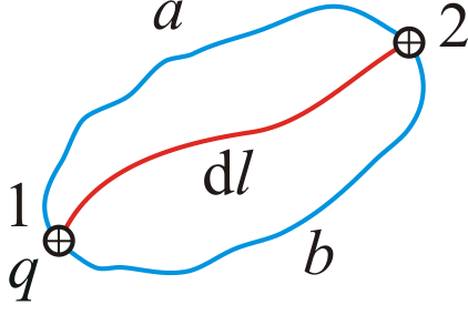
Figure 3.2.

It follows from the above that

(The integrals in the module are equal, but signs are opposite). Then work on the closed path:

(3)

or

(4)

The field with such properties is called potential . Any electrostatic field is potential.

The circulation theorem makes it possible to make a number of important conclusions, practically without resorting to calculations. Consider two simple examples confirming this conclusion.

We use the Stokes Theorem, which states that the circulation of the vector on arbitrary contour L. equal to the flow of the rotor of this vector through any surface stretched to this circuit, i.e.

. In the case of an electrostatic field we have

, so because of the arbitrariness of the surface of the surface we will get

. Consequently, from the potential nature of the electrostatic field, it follows that the electrostatic field is not vortex if . (5)

3.3. Potential energy and potential of the electrostatic field

The body in the field of potential forces has potential energy, at the expense of the work of the field. Consequently, work can be represented as a difference of values. potential energieswho possesses charge q." At points 1 and 2 fields of charge q.

Can also be shown that since

,

From here for the potential energy charge in the charge field q. We get:

(6)

Value const. in (6) are usually chosen in such a way that when the charge is removed q." infinity (

) Potential energy appealed to zero. Under this condition it turns out that

(7)

We assume q." Trial charge. Then the potential energy, which has a trial charge, depends not only on its value , but also from the value q. and r.defining the field. Therefore, this energy can be used to describe the field, just as the force acting on the trial charge was used for this purpose.

Different trial charges

,

will possess in the same point of the field different energy

,

etc. However, the attitude

It will be for all charges the same thing. Value

(8)

Called potential Fields at this point and is used along with the field strength, to describe electric fields.

As follows from (8) the potential is numerically equal to the potential energy, which has a single field in this point positive charge.

So for potential field Point charge we get the following expression:

(9)

If the field is created by a dot charge system q. 1 , q. 2 , …, q. n. located at distances respectively r. 1 , r. 2 ,…, r. n. to the point of the field in which the charge is , then work performed by this field above charge will be equal to the algebraic amount of work of forces caused by each of the charges separately:

But each of the works equal to:

Where

distance from Charity before the initial charge position,

distance from charge to the end position of the charge.

Hence:

Comparing this expression with the ratio

We get for the potential energy charge in the charge system field Expression:

, (10)

. (11).

Consequently, the potential of the field created by the charge system is equal to the algebraic amount of potentials created by each of the charges separately.

From the relationship

It follows the charge located at the point of the field with potential possesses potential energy

. Consequently, the work of the forces of the field above the charge can be expressed through the potential difference:

Thus, the work performed above the charge forces of the fieldis equal to the product of the charge on the potential difference in the initial and end points. If the charge from the point with the potential is removed to infinity (where, by condition, the potential is zero), the operation of the field forces will be equal to

or

,

T. E, potential numerical equal to workwhich field forces make a single positive charge when removing it from this field point to infinity, or the work that should be made against the electric field forces in order to move a single positive charge from infinity at this field.

For a unit of potential, a potential should be taken at such a point of the field, to move the charge to which, from infinity, it is necessary to make a job equal to

1 joule (System Units "SI")

From here

.

3.4. Dipole in the electrostatic field

E. lETTRIC DIPOLEM. Called a combination of two equal charge charges of the opposite sign that are from each other at a distance l., small compared to their distance to the points in which the dipole field is determined.

Distance between charges p \u003d.qL called dipole Moment . To complete the definition of the dipole, it is also necessary to set the orientation of the axis of the dipole in space. In accordance with this, the dipole moment should be considered as vector . This vector is attributed to the direction from negative charge to positive (Fig.3.3). If you enter a radius - vector conducted from - q. K +. q.The dipole moment can be represented as:

. (13)

If the dipole is placed in a homogeneous electric field forming dipole charges - q. and +. q. will be under the action of equal in magnitude, but opposite to the direction of forces and (Fig. 14). These forces form a couple of strength, whose shoulder is equal

That is, depends on the orientation of the dipole relative to the field. The module of each of the forces is equal qE. Multipling it on the shoulder, we get the value of the moment of the pair of the forces acting on the dipole:

Where r- The electric moment of the dipole.

IN Vector:

. (15)

Moment

seeks to turn the dipole so that his moment Installed in the direction of the field.

To increase the angle between vectors and on the dα. It is necessary to work against the forces acting on the dipole:

This work goes to an increase in potential energy. W.which is the dipole in the electric field, i.e.:

(16)

Integration (16) gives the potential energy of the dipole in the electric field expression:

Believed const.=0 , get

IN wheel const.=0 , We believe that the dipole energy will be zero when the dipole is mounted perpendicular to the field direction. The smallest value of energy equal to ( -re), it turns out when the dipole orientation in the field direction is the greatest equal rewhen directed to the side opposite to the direction of the vector .

In an inhomogeneous field, the forces acting on the dipole charges are not the same. With small size dipole f. 1 I. f. 2 can be considered approximately collinear. Suppose the field varies faster in the direction h.coinciding with the direction In the place where the dipole is located (Fig. 3.5). The positive charge of the dipole is shifted relative to the negative towards h. By magnitude

. Therefore, the field strength at points where charges are placed, differs on Δ E.. Since the amount of forces

and

or , (19)

, (20)

Where

- Electric field tension vector gradient. Thus, in an inhomogeneous electric field, except for the rotating moment, the force acts f. Under the action of which the dipole will be either drawn into the stronger field area (α 0), or pushed out of it (α\u003e 90 0).

The expression for strength can be obtained from (18), taking into account that f.= –

.

3.5. Communication between electrostatic field tension and potential

Electric field tension - the value is numerical equal poweroperate. Potential - The value is numerically equal to the potential energy of charge. Thus, there should be a connection between these values, a similar connection between potential energy and force (i.e.

). The work of the force of the field above the charge on the segment of the path can be represented as

, And loss of the potential energy of the charge, which will occur at the same time :. Where from equality

Find:

or

, (21)

Where through An arbitrarily selected direction.

,

,

, (22)

Where

Onts coordinate axes, i.e., single vector. Vector with components

where

scalar coordinate function

called gradient Functions and indicated by the symbol

(or

where - operator recruited). Thus, the gradient of the potential:

(24)

And from (23) and (24) it follows that

(25)

Since the gradient is a vector showing the direction of the separated change of some value, the value of which varies from one point of space to the other, then the gradient of the potential (Where r.-Radius-vector) is called the vector directed towards the most rapid increase in the potential, numerically equal to the speed of its change per unit length in this direction.

Insofar as

- Vector quantity, then its module is expressed as:

, (26)

Just like the vector module :

(27)

The sign "-" (25) indicates that tensions are directed toward the decrease in the potential. Formula (25) allows for known values \u200b\u200bto find the field strength at each point or solve the inverse problem, i.e., according to the specified values \u200b\u200bat each point to find the potential difference between the two arbitrary points of the field.

3.6. Equipotential surfaces

The potential of the electrostatic field is a function varying from point to point. However, in any real case, the totality of points can be distinguished, the potentials of which are the same.

G. the nestrical location of the constant potential points is called the surface of equal potential or the equipotential surface.

Take a uniformly charged endless plane (Fig. 3.6). The field created by such a plane is uniformly, and the line of tension is normal to the plane. From here it follows that the work of the charge of the charge from some point IN 1 at any other point IN 2 located at the same distance from the charged surface as the point IN 1 equal to zero. Indeed, when moving some charge q. in direct IN 1 IN 2 The force acting on the charge on the side of the field will be perpendicular to the move, and, therefore, its work is zero. But this work can be presented, on the other hand, in the form:

, (28)

G. de and

- according to the potentials of points IN 1 and IN 2 . From here, since A \u003d.0, then \u003d, i.e., the potentials of points equidistant from the charged plane are the same. Thus, the surface of equal potential (equipotential surfaces) are planes parallel to the charged plane. If the plane is charged positively, the potential value decreases as it removes from the charged plane. It is obvious that the surfaces of equal potential are located symmetrically on both sides of the charged plane.

Equipotential surfaces of a point charge of this sphere with a radius r. The center of which is located in the center of the point charge, i.e.

(Fig. 3.7). In fig. 3.6 and fig. 3.7 The vector of tension is perpendicular to the equipotential surfaces.

We show that the tension vector is perpendicular to the equipotential surface. Consider work on the movement of charge on the surface of an equal potential in a small section of the path Δ S. (Fig. 3.7). At the same time, work electric power

On this path will be:

Where α is the angle between the direction of force f. and moving Δ. S.. On the other hand, this work can be expressed as a product of the magnitude of the moving charge on the potential difference in the initial and final charge positions, i.e.

.

Since the movement goes along the equipotential surface, then the potential difference

and

, or cosα \u003d 0, it means α \u003d 90 0 i.e. The angle between the direction of force and the movement Δ S. equal to 90 0. But, i.e. Directions I. coincide therefore the angle between and Δ. S., α \u003d 90 0 i.e. the direction of the electrostatic field intensity vector is always perpendicular to the equipotential surface.

Equipotential surfaces around the charged body can be conducted as much as many. In the thickness of the equipotential surfaces, one can judge the magnitude However, provided that the potential difference between two neighboring equipotential surfaces is equal to a constant value.

The formula expresses the connection of the potential with tension and allows for known values \u200b\u200bφ to find the field strength at each point. You can solve the inverse task, i.e. According to famous values \u200b\u200bat each point of the field, find the potential difference between two arbitrary points of the field. To do this, we use the fact that the work performed by the fields above the charge q. When moving it from point 1 to point 2, it can be calculated as:

On the other hand, work can be represented as:

, then

The integral can be taken along any line connecting point 1 and point 2, because The work of the forces of the field does not depend on the path.

When around a closed contour

We get:

those. Came to the well-known tension vector circulation theorem: the circulation of the tension vector of the electrostatic field along any closed circuit is zero.

The field possessing this property is called potential.

From the circulation to zero vector circulation it follows that the lines of the electrostatic field can not be closed: they start on positive charges(sources ) and on negative charges End(stoki. ) or go into infinity.

Summarizing the theorem of Gauss and the theorem on the circulation of the vector of the electrostatic field in vacuo. Since, and

T.

. Insofar as

(

- Laplace operator), then for the potential φ we get expression

or

called poisson equation.

This equation allows the charge distribution

and a given boundary condition for the potential φ determine the values

in all points of the field, and then on the formula to find tensions

Fields, i.e. Solve the direct task of electrostatics.

3.7. Calculation of the potential difference on the tension of the field of the simplest electrostatic fields

The established relationship between tensions and potential allows the field in the well-known field strength to find the potential difference between the two arbitrary points of this field.

Consider several examples of calculating the potential difference between points of the field created by some charged bodies.

1. Field uniformly charged infinite plane

The field of a uniformly charged endless plane, found using the Ostrogradsky-Gauss theorem, is determined by the formula

where σ - surface density Charge. The potential difference between dots lying at distances x. 1 and x. 2 from the plane is equal

.

d e \u003d 0, between the plates, the potential is reduced by logarithmic law, and the second occurrence (outside the cylinders) shields the electric field and φ and E. equal zero.
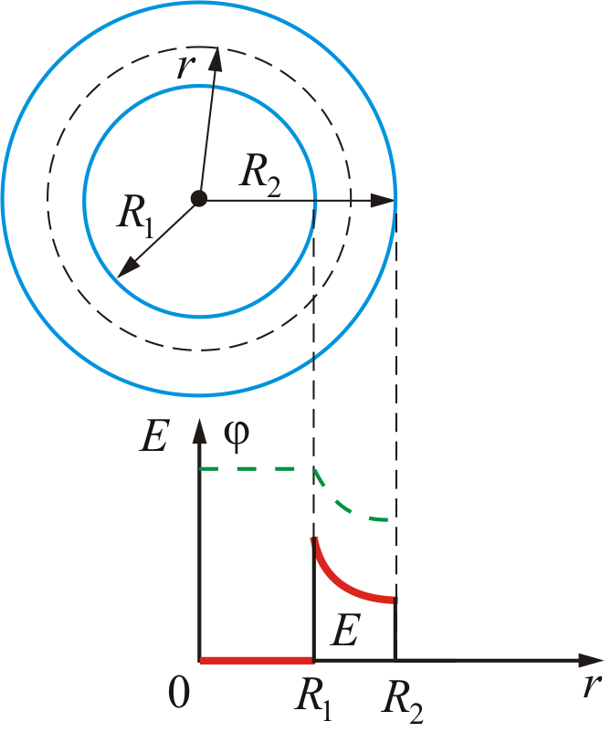
Figure 3.10
In fig. 3.10 shows the dependence of tension E. and potential from r..
4. Field of uniformly charged spherical surface
Considering examples of applying the Ostrogradsky-Gauss theorem, we found that the field strength of the sphere is determined by the formula:

(Fig. 3.11). And because

T.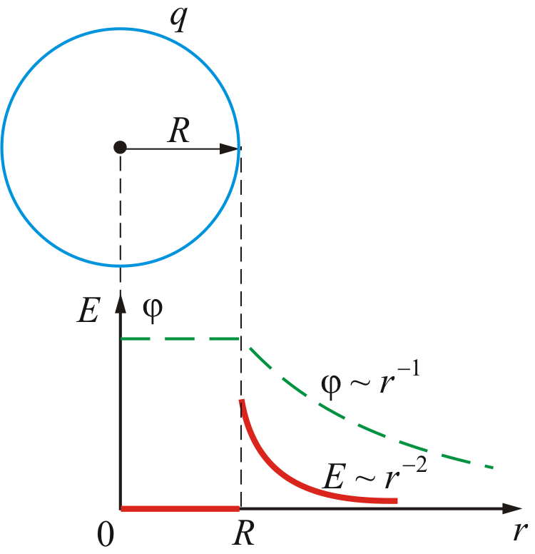

Figure 3.11
. If taken r. 1 = r. , but r. 2 =∞, the potential outside the spherical surface is determined by the expression), is determined by the formula
Score of the zero level of potential at the point r. 2 \u003d ∞ The potential of any point inside the charged ball can be found as follows:

. After integration, we get

.

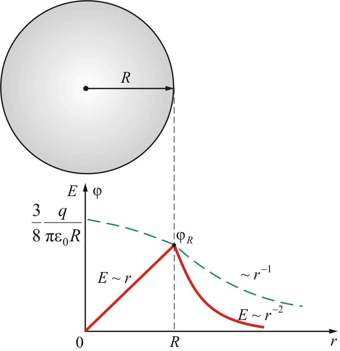
Figure 3.12
If you consider that

T.

(38 )
From the obtained relations you can do the following conclusions .
- With the help of the Gauss theorem, it is relatively simply simply to calculate E and φ from various charged surfaces.
- The field strength in vacuo varies with a jump in transition through a charged surface.
- Field potential is always a continuous function of coordinates.
Control questions
1. How to show that the electrostatic field is potentially?
2. What is the potential?
3. What is called tension vector circulation?
4. What is the connection of tension and potential? How, in the picture of the equipotential surfaces, draw a picture of the power lines of the field?
5. What is the work on the movement of the charge on the equipotential surface?
6. Give examples of calculating the difference in the potentials of the simplest electrostatic fields.
7. How does the dipole behave in the external electrostatic field?

Lecture 6. Electric field potential. Examination number 2

The potential refers to the most complex concepts of electrostatics. Students learn the definition of the potential of the electrostatic field, solve numerous tasks, but they have no sensation of the potential, they with difficulty correlate theory with reality. Therefore, the role of an educational experiment in the formation of the concept of potential is very high. We need such experiments that, on the one hand, would illustrate abstract theoretical ideas about the potential, and on the other hand, showed complete validity of the experiment of the concept of potential. To strive for the special accuracy of quantitative results in these experiments is rather harmful than useful.

6.1. Potentialness of the electrostatic field

On an insulating stand, strengthen the conductive body and charge it. On a long isolated thread, suspend a lightly conductive ball and let's notify him a trial charge, the same name with the body charge. The ball will pushes from the body and from the position 1 will turn to the Regulation 2. Since the height of the ball in the field of gravity increased by h., the potential energy of its interaction with Earth has increased mGH. So, the electrical field of the charged body made some job over a test charge.

We repeat the experience, but at the initial moment you will not just let go of a trial ball, and I spread it in an arbitrary direction, informing him of some kinetic energy. In this case, find what moves from the position 1 on a complex trajectory, the ball will eventually stop in the position 2 . Reported ball at the initial moment kinetic energyObviously, he was spent on overcoming friction forces when the ball moves, and the electric field made the same job over the ball as in the first case. In fact, if you remove the charged body, the same push of the trial ball leads to the fact that 2 He returns to position 1 .

Thus, experience suggests that the work of the electric field above the charge does not depend on the trajectory of the charge of the charge, but is determined only by the provisions of its initial and endpoints. In other words, on a closed trajectory, the operation of the electrostatic field is always equal to zero. Fields possessing such a property called potential.

6.2. The potentiality of the central field

Experience shows that in the electrostatic field created by the charged conductive ball, the force acting on the trial charge is always directed from the center of the charged ball, it monotonously decreases with increasing distance and equal distances from it has the same values. This field is called central. Using the drawing, it is easy to make sure that the central field is potentially.

6.3. Potential charge energy in the electrostatic field

Gravitational field, like electrostatic, potentially. In addition, the mathematical record of the law of world gravity coincides with the record of the law of Kulon. Therefore, in the study of the electrostatic field, it makes sense to rely on an analogy between gravitational and electrostatic fields.

In a small area near the surface of the Earth, the gravitational field can be considered homogeneous (Fig. but).

On the body weighing M in this field there is a constant module and the direction of force f. \u003d T. g.. If the body provided himself falls out of position 1 in the Regulation 2 , then the strength of gravity makes work A. = fS. = mGS. = mG. (h. 1 – h. 2).

This is the same we can say otherwise. When the body was in position 1 , the system of the earth-body possessed potential energy (i.e. the ability to work) W. 1 = mGH one . When the body passed into position 2 The system under consideration began to possess potential energy W. 2 = mGH 2. The work performed at the same time is equal to the difference in the potential energies of the system in the final and initial states taken with the opposite sign: BUT = – (W. 2 – W. 1).

We now turn to the electric field, which, recall, like gravitational, is potential. Imagine that there is no gravity forces, and instead of the surface of the Earth, there is a flat conductive plate, charged (for definiteness) negatively (Fig. b.). We introduce the coordinate axis Y. and over the plate bypass positive charge q.. It is clear that because the charge itself does not exist, over the plate there is some kind of body of a certain mass carrying an electrical charge. But, since we consider the field of gravity absent, then we will not take into account the mass of the charged body.

So, on a positive charge q. From the side of the negatively charged plane there is an attraction force f. = q. E. where E. - Electric field strength. Since the electric field is uniformly, then at all its points there is one and the same force. If the charge is moved from the position 1 in the Regulation 2 , the electrostatic force makes it easy to work BUT = fS. = qE S. = qE(y. 1 – y. 2).

We can express the same in other words. Pregnant 1 located in the electrostatic field charge possessed potential energy W. 1 = qey. 1, and in position 2 - potential energy W. 2 = qey. 2. When switching the charge 1 in the Regulation 2 The electric field of the charged plane accumulated work BUT = –(W. 2 – W. 1).

Recall that the potential energy is determined only with accuracy to the terms: if the zero value of potential energy to choose in another place of the axis Y., in principle, nothing will change.

6.4. The potential of a homogeneous electrostatic field

If the potential charge energy in the electrostatic field is divided into the magnitude of this charge, then we obtain the energy characteristics of the field itself called potential:

The potential in the SI system is expressed in volta.: 1 V \u003d 1 J / 1 CL.

If in a homogeneous electric field axis Y. send parallel to the voltage vector E. , The potential of an arbitrary point of the field will be proportional to the coordinate of the point: and the coefficient of proportionality is the voltage of the electric field.

6.5. Potential difference

Potential energy and potential are determined only with an accuracy of an arbitrary constant, depending on the choice of their zero values. However, the field operation has a completely definite value, since it is determined by the difference of potential energies at two points of the field:

BUT = –(W. 2 – W. 1) = –( 2 q. – 1 q.) = q.( 1 – 2).

Work on the movement of the electric charge between the two points of the field is equal to the product of the charge on the potential difference of the initial and endpoints. Potential difference is different called voltage.

The voltage between the two points is equal to the attitude of the field when the charge is moved from the starting point to the final charge to this:

Voltage, like the potential, is expressed in Volta.

6.6. Potentials and tension

In a uniform electric field, the tension is directed toward the decrease in the potential and, according to the formula \u003d EY., potential difference is equal U. = 1 – 2 = E.(w. 1 – y. 2). Designating the difference in the coordinates of the points w. 1 – y. 2 = d.Receive U. = ED.

In the experiment, instead of direct measurement of tension, it is easier to determine the potential difference and then calculate the voltage modulus by the formula

where d. - distance between two points of the field closely located in the direction of the vector E. . At the same time, not newton on the pendant is used as a unit of voltage, but volts per meter:

6.7. The potential of an arbitrary electrostatic field

Experience shows that the ratio of work on the movement of charge from infinity at this field point to the magnitude of this charge remains unchanged: \u003d BUT/q.. This relationship is called called potential of this point of the electrostatic field, taking the potential in infinity equal to zero.

6.8. Superposition principle for potentials

6.9. Potential Pattern Point Charge

We now turn to spherical (point) charge. It is shown above that the tension of the electric field created by uniformly distributed in the sphere of charge Q., does not depend on the radius of the sphere. Imagine that at some distance R. From the center of the sphere is a trial charge q.. The intensity of the field at the point where the charge is

The figure shows a graph of the dependence of the force of electrostatic interaction between the point charges from the distance between them. To find the work of the electric field when moving the test charge q. With distance r. up to distance R., disarm this gap dots r. 1 , r. 2 ,..., r P. on equal segments. The average force acting on the charge q. within the segment [ rR 1], equal

The work of this force on this site:

Similar expressions for work will be obtained for all other sections. Therefore, full work:

The same terms are destroyed with opposite signs, and we finally get:

- work fields above charge

- Potential difference

Now, to find the potential of the point of the field regarding infinity, ascertain R. To infinity and finally get:

So, the potential of the point of the point charge is inversely proportional to the distance to charge.

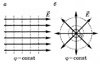
6.10. Equipotential surfaces

The surface at each point of which the potential of the electric field has the same value, called equipotential. Equipotential surfaces of the charged ball field is easy to demonstrate a test charge suspended on the thread, as shown in the figure.

In the second figure, the electrostatic field of two different charges is represented by force (solid) and equipotential (dashed) lines.

Study 6.1. Potential difference

The task. Develop a simple experience that allows you to introduce the concept of potential difference, or voltage.

Execution option. Two metal disks on insulating stands, install parallel to each other at a distance of about 10 cm. Discs Charge equal to the module and opposite by the charge sign. Charge the ball of electrostatic dynamometer charge, for example, q. \u003d 5 ND (see Study 3.6), and enter it into the area between the disks. In this case, the dynamometer arrow will show a definite value of the force acting on the ball. Knowing the dynamometer parameters, calculate the value of the force module (see Study 3.6). For example, in one of our experiments, the dynamometer arrow showed the value h. \u003d 2 cm, therefore, according to the formula, the power module f. = Kh. \u003d 17 10 -5 N.

By moving the dynamometer, show that at all points of the field between charged discs on the trial charge there is the same force. By moving a dynamometer so that the trial charge passes the way s. \u003d 5 cm in the direction of force acting on it, ask students: What kind of work does the electric field do? Achieve understanding that the field work above the charge in the module is equal

BUT = fS. \u003d 8.5 10 -6 J, (6.3)

moreover, it is positive if the charge moves in the direction of the field strength, and is negative, if in the opposite direction. Calculate the potential difference between the initial and end positions of the dynamometer ball: U. = BUT/q. \u003d 1.7 10 3 V.

On the one hand, the tension of the electric field between the plates:

On the other hand, according to formula (6.1), d \u003d S.:

Thus, experience shows that the voltage of the electric field can be determined in two ways that, of course, lead to the same results.

Study 6.2. Conditioning Electrometer for Voltage

The task. Develop an experiment showing that with the help of a demonstration switching electrometer, a voltage can be measured.

Execution option. Experimental installation is schematically shown in the figure. Using an electrostatic dynamometer, determine the tension of a homogeneous electric field and by the formula U \u003d ED. Calculate the potential difference between the conductive plates. Repeating these actions, reward the voltage electrometer so that an electrostatic voltmeter is turned out.

Study 6.3. Potential of the field of spherical charge

The task. Experimentally determine the work that needs to be performed against the electrostatic field to move the test charge from infinity into some point of the field created by the charged sphere.

Execution option. On an insulating rack, fasten the bulb from the foam wrapped by an aluminum foil. Charge it from a piezoelectric or other source (cm. Section 1.10) and charge the test ball at the electrostatic dynamometer terminal. The trial charge is infinitely far from the studied if the electrostatic dynamometer does not record the forces of electrostatic interaction between charges. In the experiment, the electrostatic dynamometer is convenient to leave fixed, and move the charge under study.

Gradually bring the charged ball on an insulating stand to an electrostatic dynamometer ball. In the first string of the table, write down the distance values r. Between charges, in the second line - the corresponding values \u200b\u200bof the power of electrostatic interaction. It is convenient to express the distance in centimeters, and the force in the conventional units in which the dynamometer scale will be separated. According to the resulting data, build a graph of power dependence on distance. You have already built a similar schedule, performing a study 3.5.

Now find the dependence of work on the movement of the charge from infinity at this field. Note that in the experiment, the strength of the interaction of charges becomes almost equal to zero on a relatively small removal of one charge from the other.

We break the entire range of distance change between charges on equal sections, for example, 1 cm. Experimental data processing is more convenient to start from the end of the graph. On the plot from 16 to 12 cm. The average value of power f. CP is 0.13 SL. units, so elementary work BUT In this area is 0.52 SL. units. On a plot from 12 to 10 cm, arguing in a similar way, we obtain the elementary operation of 0.56 conditions. units. Further, it is convenient to take plots with a length of 1 cm. On each of them, find the average value of the power and multiply it to the length of the site. Field work values A. At all areas, bring the table in the fourth line.

To find out the job BUTaccomplished by an electric field when you move the charge from infinity at this distance, fold the corresponding elementary work and the resulting values \u200b\u200bare recorded in the fifth line of the table. In the last line, write down the values \u200b\u200bof 1 / r., reverse distance between charges.

Build a graph of the dependence of the electric field from the size, reverse distance, and make sure that the straight line is obtained (figure on the right).

Thus, experience shows that the operation of the electric field when the charge of the charge from infinity at this point of the field is inversely proportional to the distance from this point to charge that creates the field.

Study 6.4. High voltage voltage source

Information. For a school physical experiment, the industry currently produces excellent high voltage sources. They have two output terminals or two high-voltage electrodes, the potential difference between which is smoothly adjustable from 0 to 25 square meters. The device built into the instrument or digital voltage meter allows you to determine the potential difference between the source poles. Such devices increase the level of the ethnostatic learning experiment.

The task. Develop an evidential training experiment showing that the potential of the charged ball, experimentally determined in accordance with formula (6.2) for a point charge, is equal to the potential reported to this ball by a high-voltage power source.

Execution option. Collect an experimental setting consisting of an electrostatic dynamometer with a test ball and conductive ball on an insulating stand (see Research 3.4 and 6.3). Measure the parameters of all installation elements.

For definiteness, we indicate that in one of the experiments we used an electrostatic dynamometer, the parameters of which are indicated in the study 3.4: but \u003d 5 10 -3 m, b. \u003d 55 10 -3 m, from \u003d 100 10 -3 m, t. \u003d 0.94 10 -3 kg, and the balls were the same and had a radius R. \u003d 7.5 10 -3 m. For this dynamometer, calibration coefficient K., transferring conditional units of strength to Newtons, is given by the formula (cm. Study 3.6).

The schedule for moving the trial charge from infinity at this field is shown in the figure on C. 31. In order to go to Joules in this graphics from conditional units, it is necessary in accordance with the formula A. = f. cf. r. Distance values \u200b\u200bin centimeters Translate to meters, power values \u200b\u200bin conditions. units. (cm) Translate into SL. units. (m) and multiply K.. In this way: A. (J) \u003d 10 -4 K.A. (Ubed. Ed.).

The corresponding graph of the dependence of work from the value, reverse distance, is presented below. Extrapolating it to R. \u003d 7.5 mm, we get that work on moving the test charge from infinity to the surface of the charged ball BUT \u003d 57 10 -4 k \u003d 4.8 10 -5 j. Since the charges of the balls were the same and accounted for q. \u003d 6.6 10 -9 CL (see Study 3.6), then the required potential \u003d BUT/q. \u003d 7300 V.

Turn on the high-voltage source and adjust the output voltage on it, for example, U. \u003d 15 sq. M. One of the electrodes is alternately touched to the conducting balls and turn off the source. At the same time, each of the balls acquires relative to the ground potential \u003d 7.5 square meters. Repeat the experience to determine the charges of balls by the Coulomb (study 3.6) and you will get a value close to 7 ND.

Thus, in the experiment, two independent methods are determined balls of balls. The first method is based on the direct use of the determination of the potential, the second is based on the message to the balls of a certain potential with the help of a high-voltage source and the subsequent measurement of their charge using the Culon law. It turned out coincident results.

Of course, none of the schoolchildren does not doubt that modern devices correctly measure the values \u200b\u200bof physical quantities. But now they are convinced that they are correctly measured by those values \u200b\u200bthat they are studied in the simplest phenomena. There is a strong bond between the basics of physics and modern technique, the abyss between school knowledge and real life is eliminated.

Questions and tasks for self-control

1. How to experimentally prove that the electrostatic field is potentially?

2. What is the essence of an analogy between gravitational and electrostatic fields?

3. What is the connection between the voltage and the difference between the potentials of the electrostatic field?

4. Invite the experience of directly justifying the justice of the principle of superposition for potentials.

5. Calculate the potential of the point charge field, using integral calculus. Compare the output of the formula with the elementary conclusion given in the lecture.

6. Find out why in the experience in determining the difference in potentials between two conductive disks (Study 6.1) You cannot move the tension meter so that its trial ball has passed all the distance from one disk to another.

7. Removing the voltage electrometer (study 6.2), compare the resulting result with the values \u200b\u200bof the sensitivity of the voltage device, which are given in the passport data of the electroometer.

9. Develop in detail the methodology of formation in the consciousness of students of the reasonable conviction that the concept of the electric field potential introduced in the study of electrostatics is accurately complies with the one that is used modern science and technique.

Literature

Butikov E.I., Kondratyev A.S. Physics: studies. Manual: 3 kN. Kn. 2. Electrodynamics. Optics. - M.: Fizmatlit, 2004.

Voskanyan A.G.., Marlensky A.D., Shibayev A.F. Demonstration of the Culon Law on the basis of quantitative measurements: in Sat. "Educational experiment on electrodynamics", vol. 7. - M.: School press, 1996.

Kasyanov V.A. Physics-10. - M.: Drop, 2003.

Myakyshev G.Ya., Synyakov A.Z.., Slobodskov B.A.. Physics: electrodynamics. 10-11 kl.: Studies. For corner. Study of physics. - M.: Drop, 2002.

Educational equipment for physics Cabinets educational institutions: Ed. G.G.Nikorov. - M.: Drop, 2005.